The symmetrized Fermi function and its transforms

Symmetrized Fermi function 6531
By reversing the order of summations we have
∞∑ ∞∑
q 2 v(q) = 2
(−) l lC p c 2l α 2l . (39)
p=1
y p−1
p=0 l=p
The coefficient of y p−1 can be expressed in closed form if we note from equation (37)
(with D = 1) that
α 2p ( ) ∂ p
α
∞∑
p! ∂α 2 sinh α = (−) l c 2ll C p α 2l . (40)
l=p
Thus,
q 2 α
∞∑
v(q) − zJ 1 (z)
sinh α = 1 ∂ p α
y p−1
p! α2p ∂(α
p=1
2 ) p sinh α
∞∑
( )
1 1 ∂ p
α
= y p−1
2 p p! α2p α ∂α sinh α
)
∂ p
α
∂α sinh α . (41)
∞∑
(
p
(2p − 3)!! J p−1 (z) 1
= (−) α 2p
2
p=1
p p! z p−1 α
We worked out the first few terms of this series explicitly, with the result
q 2 v(q) =
πqd [
qRJ 1 (qR) + 1 ( )
πqd
sinh πqd
2 tanh πqd −1 J 0 (qR)
+ 1 [( )(
) ] 2πqd
πqd
8 tanh πqd +1 tanh πqd −1 −(πqd) 2 J1 (qR)
qR
+ 1 [ ( 2(πqd)
2
3
16 tanh 2 πqd + 2πqd )(
)
πqd
tanh πqd +1 tanh πqd −1
− 5(πqd)3
tanh πqd
× J 2(qR)
(qR) 2 +···]
. (42)
It is seen that α/ sinh α is a common factor, and the remaining coefficients become
polynomials in α at large qd, soq 2 v(q) decreases exponentially. The coefficients of y p
become more and more complicated but one can certainly work them out systematically.
The result is an asymptotic series in z, where the dependence on α has been summed. One
is not limited to small qd, as for the Sommerfeld expansion, or equation (31). On the other
hand, if equation (42) is expanded in powers of α, it reproduces exactly equation (31).
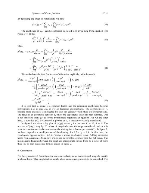
In figure 1 we show a log plot of |v(q)| versus q for the case R = 30, d = 1. The
maxima of |v(q)| vary by 20 orders of magnitude over the range considered, and on this
scale the exact (numerical) values cannot be distinguished from expression (42). In figure 2,
we have expanded a small portion of the drawing, for 2.2