Numerical solution of the Schrödinger equation

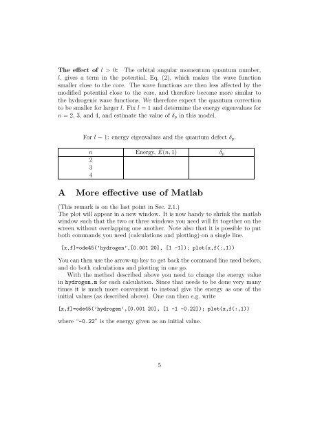
The effect of l > 0: The orbital angular momentum quantum number,
l, gives a term in the potential, Eq. (2), which makes the wave function
smaller close to the core. The wave functions are then less affected by the
modified potential close to the core, and therefore become more similar to
the hydrogenic wave functions. We therefore expect the quantum correction
to be smaller for larger l. Fix l = 1 and determine the energy eigenvalues for
n = 2, 3, and 4, and estimate the value of δ p in this model.
For l = 1: energy eigenvalues and the quantum defect δ p .
n Energy, Ẽ(n,1) δ p
2
3
4
A More effective use of Matlab
(This remark is on the last point in Sec. 2.1.)
The plot will appear in a new window. It is now handy to shrink the matlab
window such that the two or three windows you need will fit together on the
screen without overlapping one another. Note also that it is possible to put
both commands you need (calculations and plotting) on a single line.
[x,f]=ode45(’hydrogen’,[0.001 20], [1 -1]); plot(x,f(:,1))
Youcanthenuse the arrow-upkey to get back thecommand lineused before,
and do both calculations and plotting in one go.
With the method described above you need to change the energy value
in hydrogen.m for each calculation. Since that needs to be done very many
times it is much more convenient to instead give the energy as one of the
initial values (as described above). One can then e.g. write
[x,f]=ode45(’hydrogen’,[0.001 20], [1 -1 -0.22]); plot(x,f(:,1))
where “-0.22” is the energy given as an initial value.
5