Twenty Years of Linear Programming Based Portfolio Optimization
Twenty Years of Linear Programming Based Portfolio Optimization
Twenty Years of Linear Programming Based Portfolio Optimization

Create successful ePaper yourself
Turn your PDF publications into a flip-book with our unique Google optimized e-Paper software.
R. Mansini et al. / European Journal <strong>of</strong> Operational Research 234 (2014) 518–535 525<br />
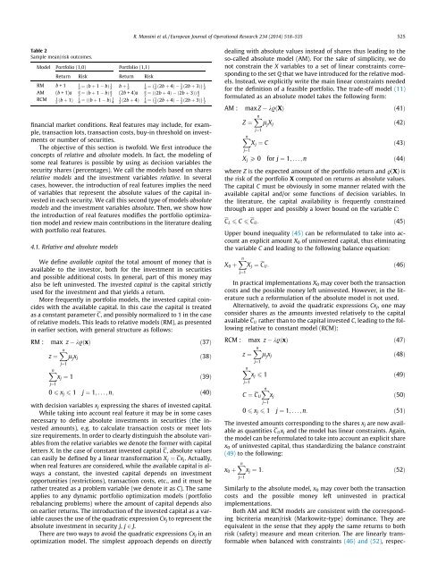
Table 2<br />
Sample mean/risk outcomes.<br />
Model <strong>Portfolio</strong> (1,0) <strong>Portfolio</strong> (1,1)<br />
Return Risk Return Risk<br />
RM b +1 1<br />
2 ¼ðb þ 1 bÞ 1 2 b þ 1 2<br />
AM (b +1)a a<br />
2 ¼ðb þ 1 bÞ a 2 (2b +4)a a<br />
RCM 1 2 ðb þ 1Þ 1<br />
4 ¼ððb þ 1 bÞ 1 4<br />
financial market conditions. Real features may include, for example,<br />
transaction lots, transaction costs, buy-in threshold on investments<br />
or number <strong>of</strong> securities.<br />
The objective <strong>of</strong> this section is tw<strong>of</strong>old. We first introduce the<br />
concepts <strong>of</strong> relative and absolute models. In fact, the modeling <strong>of</strong><br />
some real features is possible by using as decision variables the<br />
security shares (percentages). We call the models based on shares<br />
relative models and the investment variables relative. In several<br />
cases, however, the introduction <strong>of</strong> real features implies the need<br />
<strong>of</strong> variables that represent the absolute values <strong>of</strong> the capital invested<br />
in each security. We call this second type <strong>of</strong> models absolute<br />
models and the investment variables absolute. Then, we show how<br />
the introduction <strong>of</strong> real features modifies the portfolio optimization<br />
model and review main contributions in the literature dealing<br />
with portfolio real features.<br />
4.1. Relative and absolute models<br />
We define available capital the total amount <strong>of</strong> money that is<br />
available to the investor, both for the investment in securities<br />
and possible additional costs. In general, part <strong>of</strong> this money may<br />
also be left uninvested. The invested capital is the capital strictly<br />
used for the investment and that yields a return.<br />
More frequently in portfolio models, the invested capital coincides<br />
with the available capital. In this case the capital is treated<br />
as a constant parameter C, and possibly normalized to 1 in the case<br />
<strong>of</strong> relative models. This leads to relative models (RM), as presented<br />
in earlier section, with general structure as follows:<br />
RM : max z k.ðxÞ ð37Þ<br />
z ¼ Xn<br />
l j<br />
x j<br />
ð38Þ<br />
X n<br />
j¼1<br />
j¼1<br />
x j ¼ 1<br />
1<br />
4 ¼ 1 2 ð2b þ 4Þ 1<br />
2 ð2b þ 3Þ 1<br />
2<br />
2 ¼ðð2b þ 4Þ ð2b þ 3ÞÞ a 2<br />
1<br />
2 ð2b þ 4Þ 1<br />
4 ¼ 1 2 ð2b þ 4Þ 1<br />
2 ð2b þ 3Þ 1<br />
2<br />
ð39Þ<br />
0 6 x j 6 1 j ¼ 1; ...; n; ð40Þ<br />
with decision variables x j expressing the shares <strong>of</strong> invested capital.<br />
While taking into account real feature it may be in some cases<br />
necessary to define absolute investments in securities (the invested<br />
amounts), e.g. to calculate transaction costs or meet lots<br />
size requirements. In order to clearly distinguish the absolute variables<br />
from the relative variables we denote the former with capital<br />
letters X. In the case <strong>of</strong> constant invested capital C, absolute values<br />
can easily be defined by a linear transformation X j ¼ Cx j . Actually,<br />
when real features are considered, while the available capital is always<br />
a constant, the invested capital depends on investment<br />
opportunities (restrictions), transaction costs, etc., and it must be<br />
rather treated as a problem variable (we denote it as C). The same<br />
applies to any dynamic portfolio optimization models (portfolio<br />
rebalancing problems) where the amount <strong>of</strong> capital depends also<br />
on earlier returns. The introduction <strong>of</strong> the invested capital as a variable<br />
causes the use <strong>of</strong> the quadratic expression Cx j to represent the<br />
absolute investment in security j, j 2 J.<br />
There are two ways to avoid the quadratic expressions Cx j in an<br />
optimization model. The simplest approach depends on directly<br />
dealing with absolute values instead <strong>of</strong> shares thus leading to the<br />
so-called absolute model (AM). For the sake <strong>of</strong> simplicity, we do<br />
not constrain the X variables to a set <strong>of</strong> linear constraints corresponding<br />
to the set Q that we have introduced for the relative models.<br />
Instead, we explicitly write the main linear constraints needed<br />
for the definition <strong>of</strong> a feasible portfolio. The trade-<strong>of</strong>f model (11)<br />
formulated as an absolute model takes the following form:<br />
AM : max Z k.ðXÞ ð41Þ<br />
Z ¼ Xn<br />
l j<br />
X j<br />
ð42Þ<br />
X n<br />
j¼1<br />
j¼1<br />
X j ¼ C<br />
ð43Þ<br />
X j P 0 for j ¼ 1; ...; n ð44Þ<br />
where Z is the expected amount <strong>of</strong> the portfolio return and .(X) is<br />
the risk <strong>of</strong> the portfolio X computed on returns as absolute values.<br />
The capital C must be obviously in some manner related with the<br />
available capital and/or some functions <strong>of</strong> decision variables. In<br />
the literature, the capital availability is frequently constrained<br />
through an upper and possibly a lower bound on the variable C:<br />
C L 6 C 6 C U :<br />
ð45Þ<br />
Upper bound inequality (45) can be reformulated to take into account<br />
an explicit amount X 0 <strong>of</strong> uninvested capital, thus eliminating<br />
the variable C and leading to the following balance equation:<br />
X 0 þ Xn<br />
X j ¼ C U :<br />
j¼1<br />
ð46Þ<br />
In practical implementations X 0 may cover both the transaction<br />
costs and the possible money left uninvested. However, in the literature<br />
such a reformulation <strong>of</strong> the absolute model is not used.<br />
Alternatively, to avoid the quadratic expressions Cx j , one may<br />
consider shares as the amounts invested relatively to the capital<br />
available C U rather than to the capital invested C, leading to the following<br />
relative to constant model (RCM):<br />
RCM : max z k.ðxÞ ð47Þ<br />
z ¼ Xn<br />
l j<br />
x j<br />
ð48Þ<br />
X n<br />
j¼1<br />
j¼1<br />
x j 6 1<br />
C ¼ C U<br />
X n<br />
j¼1<br />
x j<br />
ð49Þ<br />
ð50Þ<br />
0 6 x j 6 1 j ¼ 1; ...; n: ð51Þ<br />
The invested amounts corresponding to the shares x j are now available<br />
as quantities C U x j and the model has linear constraints. Again,<br />
the model can be reformulated to take into account an explicit share<br />
x 0 <strong>of</strong> uninvested capital, thus standardizing the balance constraint<br />
(49) to the following:<br />
x 0 þ Xn<br />
x j ¼ 1:<br />
j¼1<br />
ð52Þ<br />
Similarly to the absolute model, x 0 may cover both the transaction<br />
costs and the possible money left uninvested in practical<br />
implementations.<br />
Both AM and RCM models are consistent with the corresponding<br />
bicriteria mean/risk (Markowitz-type) dominance. They are<br />
equivalent in the sense that they apply the same returns to both<br />
risk (safety) measure and mean criterion. The are linearly transformable<br />
when balanced with constraints (46) and (52), respec-