Multi-Threaded Fluid Simulation
Multi-Threaded Fluid Simulation
Multi-Threaded Fluid Simulation

Create successful ePaper yourself
Turn your PDF publications into a flip-book with our unique Google optimized e-Paper software.
MULTI-THREADED FLUID SIMULATION FOR GAMES<br />
The main computational load of the simulation occurs<br />
when each step loops over the grid. These are all nested<br />
loops, so a straightforward way to break them up is by<br />
using the “parallel for” construction of TBB. In the example<br />
case of density diffusion, the code went from the serial<br />
version shown in Figure 3 to the parallel version shown in<br />
Figures 5 and 6.<br />
Figure 5. Using Intel® Threading Building Blocks to call the<br />
diffusion algorithm.<br />
Figure 4. Breaking up a 2D grid into tasks and an individual cell<br />
adjacent to other tasks<br />
For example, in the simulation there is a diffusion step<br />
followed by a force update step and later, an advection<br />
step. At each step the grid is broken into pieces, and the<br />
tasks write their data to a shared output grid, which<br />
becomes the input into the next step. In most cases, this<br />
approach works well. However, a problem can arise if the<br />
calculation uses its own results in the current step. That<br />
is, the output of cell 1 is used to calculate cell 2. Looking<br />
at Figure 4, it is obvious that certain cells, like the shaded<br />
cell, will be processed in a task separate from the task<br />
in which their immediate neighbors are processed. Since<br />
each task uses the same input, the neighboring cells’ data<br />
will be different in the multi-threaded version compared<br />
to the serial version. Whether this is an issue depends on<br />
which portion of the simulation we are in. Inaccuracies in<br />
the results in the diffusion step can occur, but they are not<br />
noticeable and don’t introduce destabilizing effects. In most<br />
cases the inaccuracies are smoothed out by subsequent<br />
iterations over the data and have no lasting impact on the<br />
simulation. This kind of behavior is acceptable because the<br />
primary concern is visual appeal, not numerical accuracy.<br />
However, in other cases inaccuracies can accumulate,<br />
introducing a destabilizing effect on the simulation, which<br />
can quickly destroy any semblance of normal behavior. An<br />
example of this occurs while processing the edge cases in<br />
diffusion—where diffusion is calculated along the edges<br />
of the grid or cube. When run in parallel, the density does<br />
not diffuse out into the rest of the volume and instead<br />
accumulates at the edges, forming a solid border. For<br />
this situation and similar ones, we simply run that<br />
portion serially.<br />
Figure 5 shows how TBB is used to call the diffusion<br />
algorithm. The arguments uBegin and uEnd are the<br />
start and end values of the total range to process, and<br />
uGrainSize is how small to break the range into. For<br />
example, if uBegin is 0 and uEnd is 99, the total range is<br />
100 units. If uGrainSize is 10, 10 tasks will be submitted,<br />
each of which will process a range of 10.<br />
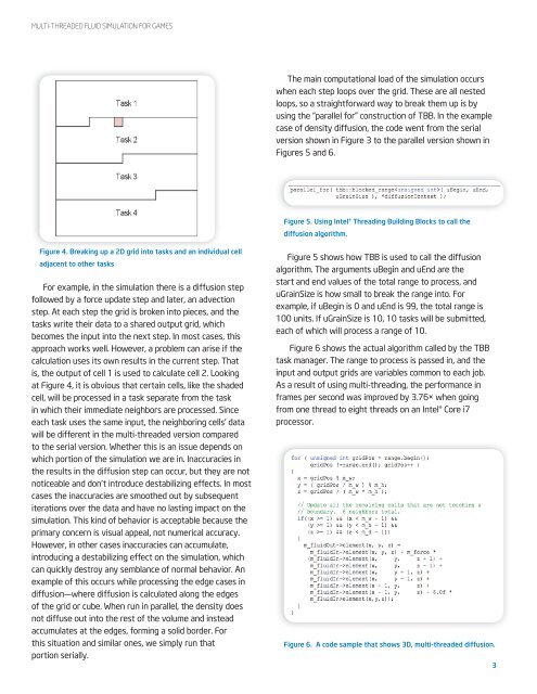
Figure 6 shows the actual algorithm called by the TBB<br />
task manager. The range to process is passed in, and the<br />
input and output grids are variables common to each job.<br />
As a result of using multi-threading, the performance in<br />
frames per second was improved by 3.76× when going<br />
from one thread to eight threads on an Intel® Core i7<br />
processor.<br />
Figure 6. A code sample that shows 3D, multi-threaded diffusion.<br />
3