METHODS FOR CALCULATING FRÉCHET DERIVATIVES AND ...

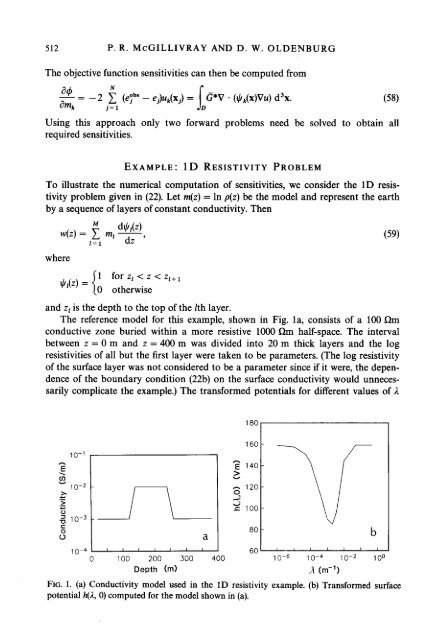
512 P. R. McGILLIVRAY AND D. W. OLDENBURGThe objective function sensitivities can then be computed fromUsing this approach only two forward problems need be solved to obtain allrequired sensitivities.EXAMPLE : 1 D RESISTIVITY PROBLEMTo illustrate the numerical computation of sensitivities, we consider the 1D resistivityproblem given in (22). Let m(z) = In p(z) be the model and represent the earthby a sequence of layers of constant conductivity. Thenwhere1 for z1 < z < z ,+~O otherwiseand zl is the depth to the top of the lth layer.The reference model for this example, shown in Fig. la, consists of a 100 Rmconductive zone buried within a more resistive 1000 Rm half-space. The intervalbetween z = O m and z = 400 m was divided into 20 m thick layers and the logresistivities of all but the first layer were taken to be parameters. (The log resistivityof the surface layer was not considered to be a parameter since if it were, the dependenceof the boundary condition (22b) on the surface conductivity would unnecessarilycomplicate the example.) The transformed potentials for different values of 1160 -hE 140->vv 2n 120-r 100-80 - bFIG. 1. (a) Conductivity model used in the 1D resistivity example. (b) Transformed surfacepotential h(l, O) computed for the model shown in (a).