Numerical Algorithm of Solving the Forced sin-Gordon Equation

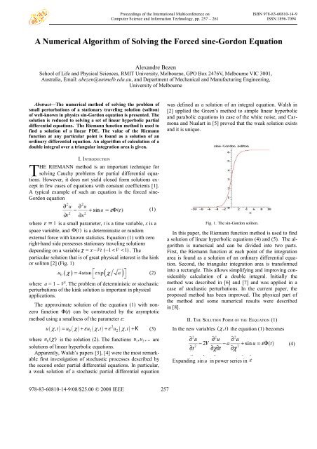
Proceedings of the International Multiconference on ISBN 978-83-60810-14-9Computer Science and Information Technology, pp. 257 – 261 ISSN 1896-7094A Numerical Algorithm of Solving the Forced sine-Gordon EquationAlexandre BezenSchool of Life and Physical Sciences, RMIT University, Melbourne, GPO Box 2476V, Melbourne VIC 3001,Australia, Email: abezen@unimelb.edu.au, and Department of Mechanical and Manufacturing Engineering,University of MelbourneAbstract—The numerical method of solving the problem ofsmall perturbations of a stationary traveling solution (soliton)of well-known in physics sin-Gordon equation is presented. Thesolution is reduced to solving a set of linear hyperbolic partialdifferential equations. The Riemann function method is used tofind a solution of a linear PDE. The value of the Riemannfunction at any particular point is found as a solution of anordinary differential equation. An algorithm of calculation of adouble integral over a triangular integration area is given.was defined as a solution of an integral equation. Walsh in[2] applied the Green’s method to simple linear hyperbolicand parabolic equations in case of the white noise, and Carmonaand Nualart in [5] proved that the weak solution existsand it is unique.TI. INTRODUCTIONHE RIEMANN method is an important technique forsolving Cauchy problems for partial differential equations.However, it does not yield closed form solutions exceptin few cases of equations with constant coefficients [1].A typical example of such an equation is the forced sine-Gordon equation(1)where ε = 1 is a small parameter, t is a time variable, x is aspace variable, and Φ ( t)is a deterministic or randomexternal force with known statistics. Equation (1) with zeroright-hand side possesses stationary traveling solutionsdepending on a variable χ = x −Vt ( − 1 < V < 1) . Theparticular solution that is of great physical interest is the kinkor soliton [2] (Fig. 1)where a = 1 – V 2 . The problem of deterministic or stochasticperturbations of the kink solution is important in physicalapplications.The approximate solution of the equation (1) with nonzerofunction Φ(t) can be constructed by the asymptoticmethod using a smallness of the parameter ε:( χ, ) ( χ ) ε ( χ, ) ε 2 ( χ,)0 1 2(2)u t = u + u t + u t +K (3)where u ( χ ) is the solution (2). The functions 0u1, u2,...aresolutions of linear hyperbolic equations.Apparently, Walsh’s papers [3], [4] were the most remarkablefirst investigation of stochastic processes described bythe second order partial differential equations. In particular,a weak solution of a stochastic partial differential equationFig. 1. The sin-Gordon soliton.In this paper, the Riemann function method is used to finda solution of linear hyperbolic equations (4) and (5). The algorithmis numerical and can be divided into two parts.First, the Riemann function at each point of the integrationarea is found as a solution of an ordinary differential equation.Second, the triangular integration area is transformedinto a rectangle. This allows simplifying and improving considerablycalculation of a double integral. Initially themethod was described in [6] and [7] and was applied in acase of stochastic perturbations. In the current paper, theproposed method has been improved. The physical part ofthe method and some numerical results were describedin [8].II. THE SOLUTION FORM OF THE EEQUATION (1)In the new variables ( χ , t)the equation (1) becomesExpanding sin u in power series in ε(4)978-83-60810-14-9/08/$25.00 © 2008 IEEE 257

258 PROCEEDINGS OF THE IMCSIT. VOLUME 3, 2008(5)Substituting (3) and (5) into (4) in the first order on εwe obtainIn the second order(6)(7)To apply the Riemann’s method of solving (6) and (7) [1]we need to transform these equations to the standard formwhich does not contain the second mixed derivative. Toget rid of the mixed derivatives let us make a transformationχ = χ V χandτ = t − . In the new variables equationsa(6) and (7) read(8)Fig .2. The function f ( χ ) , a = 1 .The corrections ui( 0 0 )0 ( 0 ) ( χ , τ )χ , τ , i = 1, 2 to the kink solutionu χ at a point 0 0 can be presented through theRiemann function ω( χ, τ ) [1]:(13)and(9)with trivial initial conditions over the straight line CVC : τ = − ξ(10)a(14)where A is the characteristic triangle in the plane ( χ, τ ),bounded by the straight line C given in (10) and the characteristicsA : τ ( χ − χ0 ) = τ10 (Fig. 3).aIII. THE RIEMANN FUNCTIONEquations (8) and (9) have the same left-hand side andcan be presented as(11)(12)wheref2( χ) 2 / cosh ( χ / a)= since1χacos[4arctan( e )] = 1−212cosh ( χ)aThe graph of the function f ( χ ) for the value V = 0.5is shown in Fig. 2.Fig. 3. The characteristic triangle A.The Riemann function ω( χ, τ ) satisfies the equation(15)with ω = 1/(2a) over the characteristics and b= a .

ALEXANDRE BEZEN: NUMERICAL ALGORITHM OF SOLVING THE FORCED SIN-GORDON EQUATION 259Since outside of a finite interval ( − χlim , χlim)then one can expect that the solution of (15) can be closeto the solution of the telegrapher’s equation [1]:1which is ω( χ, τ ) =0( )2aJ b γ and2 12γ = ( τ −τ 0) − ( χ − χ2 0) . The variable γ is a hyperbolicdistance in the characteristic triangle A . The dis-atance γ2 12is positive inside A, i.e. ( τ − τ0) > ( χ − χ2 0) ,a2 12and imaginary when ( τ − τ0) < ( χ − χ2 0) . It vanishesa2 12when ( τ − τ0) = ( χ − χ2 0) .aThe equation (15) in the variables ( χ, γ ) has the formLet’s look for the solution of (16) in the form(16)(17)where the first term of the sum is the solution of thetelegrapher’s equation and the second term must be smallfor a finite value of χlim .Since1J0 ( bγ ) + J0 ( bγ ) + J0( bγ) = 0bγthen substitution of (17) into (16) givesFor χ = χ0the last equation becomesAssumeA = 0 for odd n,AAnIt follows thatand1 f ( ξ ) 1=,02 22 a ϕ( ξ0) 2f ( ξ ) ( −1)a= [ + ( ( ) −2a 2 4 ...(2 k)bk202k+ 2ϕ ξ2 2 2 2 01(1 − f ( ξ0 )) ϕ( ξ0 )) A2 k] ,2(2k+ 2) ϕ( ξ )k = 1,2,3...Ak1 ( −1)= , k = 1,2,3...2a2 4 ...(2 k)2k+ 2 2 2 20(17)1ω( χ, γ ) = [ J0 ( bγ ) + (1 − J0( bγ )) ϕ( χ)](18)2aSubstitute (18) into (16) and we obtain that the solutionϕ( χ ) satisfies the following equation−a(1 − J ( bγ )) ϕ ( χ)+0( J ( bγ ) + J ( bγ ))( χ − χ ) ϕᄁ( χ)+0 2 0(1 − f ( χ )(1 − J ( bγ ))) ϕ( χ) = J ( bγ ) f ( χ)0 0and subject to the boundary conditionsIV. NUMERICAL ALGORITHM AND CALCULATIONS(19)(20)A solution ω( χ1, τ1)of the partial differential equation(15) at any particular point ( χ1, τ1)can be reduced tosolving the boundary value problem (19), (20) with fixedvalue of γ , where2 12γ = ( τ1 −τ 0) − ( χ2 1− χ0) .aA family of curves γ = const define hyperbolaeimbedded into the characteristic triangle (Fig.4). Thesolution surface (15) can be represented as a family ofcurves over the hyperbolae in the 3D space ( χ, τ , ω ) .The surface representing the Riemann function for χ0= 0is shown in Fig. 5 and was drawn using MAPLE.and, therefore,

260 PROCEEDINGS OF THE IMCSIT. VOLUME 3, 2008This transformation allows simplifying significantly numericalintegration and speed up the algorithm of calculationof functions u 1,2.(χ, t). The area of integration can becovered by a rectangular mesh and then, the standardSimpson method can be used [9].Fig. 4. The Characteristic triangle with the family of curvesconst γ = .Fig. 6. The rectangular integration area R(v, u).The first integral (13) in the new variables (v, u) hasthe form(21)Fig. 5. The solution surface of (15) representing the Riemannfunction. Each curve is a solution of (19), (20) for particular fixedvalue of γ .The boundary value problem (19), (20) can be solvednumerically using the relaxation method [9]. Since the solutionof this BVP approaches zero when ±∞ thenfor numerical calculations this problem can be solved forfinite values of χ which are found manually from thelimcondition .In the numerical calculations of the double integrals(13) and (14) one of the most difficult tasks is integrationover the triangle A . First, the integral needs to becalculated for various values of ( χ0, τ0). The area of therectangle A becomes larger when the value of τ0 increases.The second difficulty is that changing the value ofthe parameter a leads to changing the rectangle A shape.Therefore, it is very difficult to develop a universalalgorithm for various values of ( χ0, τ0) and the parametera . The integration area A (Fig. 3) can be mapped into awhere the double integral is calculated using the Simpsonmethod and the value of ϕ ( v, u)at each point of the integralsum is a solution of the boundary value problem(19), (20).The numerical algorithm was implemented in a programwritten in C++. For calculating values of the Besselfunctions, double integrals and solving ordinary differentialequations the code given in [9] was used.As an example, the function Φ ( t) = sin(10 t)was considered.Two graphs in a plane ( x, u1) representing resultsof calculations of the integral (21) forareshown in Fig. 7 and Fig. 8.rectangle(Fig. 6) with coordinates(v, u) by means of transformationFig. 7. V = 0.95, t = πwhere t 0= τ 0+ V χ 0/ a .

ALEXANDRE BEZEN: NUMERICAL ALGORITHM OF SOLVING THE FORCED SIN-GORDON EQUATION 261Fig. 8. V = 0, t = 4088The values of ε in (3) depend on a particular physicalproblem and are not discussed in this paper. They can beup to 0.3 in some cases.REFERENCES[1] E. Zauderer, “Partial differential equations of applied mathematics”,John Wiley & Sons Inc., USA, 1989.[2] Ablowitz MJ, Segur H. “Solitons and the Inverse Scattering Transform”,SIAM, Philadelphia, 1981.[3] J. B. Walsh, “An Introduction to stochastic partial differentialequations”, Lecture Notes in Mathematics, 1180, Springer,pp. 266-437, 1986.[4] B. Cairoli, J.B. Walsh, “Stochastic integrals in the plane”, ActaMatematica, 134, pp.111-183, 1975.[5] R. Carmona, D. Nualart, “Random non-linear wave equations:Smothness of the solutions”, Prob. Theory Rel Fields, 79,pp.469-508, 1988.[6] A. Bezen, “The Riemann’s function for a linear hyperbolic PDE”,Analysis paper, Department of Statistics, University of Melbourne,Report No 10, 1996.[7] A. Bezen, F. Klebaner, “The Riemann’s function and its applicationto stochastic perturbations of a non-linear wave equation”,Random & Computational Dynamics, 5(4), pp.307-318, 1997.[8] A. Bezen, Y. Stepanyants, “Kink propagation within the forcedsine-Gordon equation”, Proceedings of III International Conference“Frontiers of Nonlinear Physics”, Nizhny Novgorod, 3-9July, pp.50-51, 2007.[9] W. H. Press, S. A. Teukolsky, W. T. Vetterling, B. P. Flannery,“Numerical Recipes in C”, Cambridge Universiy Press, 1992.