A Comparison of Two Latency Insertion Methods in ... - IEEE Xplore

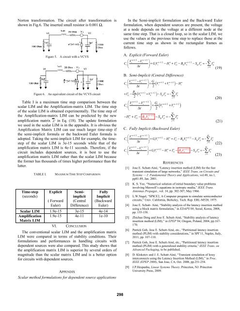
Norton transformation. The circuit after transformation isshown in Fig.6. The inserted small resistor is 0.001 Ω.Figure 5. A circuit with a VCVSFigure 6. An equivalent circuit of the VCVS circuitTable I is a maximum time step comparison between thescalar LIM and the Amplification-matrix LIM. The time stepof the scalar LIM is obtained experimentally. The time step ofthe Amplification-matrix LIM can be predicted by the newamplification matrix A ' in Eq. (18). The update formulationwe used in the scalar LIM is in the appendix. It is obvious theAmplification Matrix LIM can use much larger time-step ifthe semi-implicit formula or the backward Euler formula isadopted. Taking the semi-implicit LIM for example, the timestepof the scalar LIM is 3e-15 seconds while that of theamplification matrix LIM is 4e-11 seconds. Therefore, if thecircuit includes dependent sources, it is best to use theamplification matrix LIM rather than the scalar LIM becausethe former has thousands of times higher performance than thelatter.Time-step(seconds)TABLE I.MAXIMUM TIME STEP COMPARISONExplicit( ForwardEuler)Semiimplicit(CentralDifference)FullyImplicit(BackwardEuler)Scalar LIM 1.9e-15 3e-15 4e-14Amplification 1.9e-15 4e-11 1e-10Matrix LIMVI. CONCLUSIONThe conventional scalar LIM and the amplification matrixLIM were compared in terms of stability conditions. Theirformulations and performances in handling circuits withdependent sources were also compared. This study shows thatthe amplification matrix LIM is superior by several orders ofmagnitude than the scalar matrix LIM and is a better optionfor circuits with dependent sources.APPENDIXScalar method formulations for dependent source applicationsIn the Semi-implicit formulation and the Backward Eulerformulation, when dependent sources are present, the voltageat a node depends on the voltage at a different node at thesame time step. That is a closed loop, so in the scalar LIM, weuse the values at the previous time step to replace those at thecurrent time step as shown in the rectangular frames asfollows.A. Explicit (Forward Euler)n+ 1/2 n−1/2M⎛Vii−V⎞in−1/2 n n n−1/2n nCi⎜ ⎟+ GVi i− Hi + ILi −BikVk − SipIp = −∑ Iij⎝ Δt⎠j=1 (19)B. Semi-Implicit (Central Difference)n+ 1/2 n−1/2⎛Vi −V ⎞iGin+ 1/ 2 n−1/2nCi⎜ ⎟+ ( Vi + Vi ) −Hi⎝ Δt⎠ 2Min Bikn+ 1/2 n−1/2n n+ ILi − ( Vk + Vk ) − SipIp =−∑ Iij2j=1n+ 1/2 n−1/2⎛Vi −V ⎞iGin+ 1/2 n−1/2Ci⎜ ⎟+ ( Vi + Vi)⎝ Δt⎠ 2Min n n−1/2n n− Hi+ ILi − BikVk− SipIp=−∑ Iijj=1C. Fully Implicit (Backward Euler)(20)(21)n+ 1/2 n−1/2M⎛Vii−V⎞in+ 1/2 n n n+1/2 n nCi ⎜ ⎟+ GVi i− Hi + ILi −BikVk − SipIp =−∑ Iij⎝ Δt⎠j=1 (22)n+ 1/2 n−1/2M⎛Vii−V⎞in+1/ 2 n n n−1/2 n nCi⎜ ⎟+ GVi i− Hi + ILi − BVik k− SipIp =−∑ Iij⎝ Δt⎠j=1 (23)REFERENCES[1] Jose E. Schutt-Ainé, “Latency insertion method (LIM) for the fasttransient simulation of large networks,” IEEE Trans. on Circuits andSystems — I: Fundamental Theory and Applications, vol.48, no.1,pp81-89, Jan. 2001.[2] K. S. Yee, “Numerical solution of initial boundary value problemsinvolving Maxwell’s equations in isotropic media,” IEEE Trans.Antennas Propagat., vol. 14, pp. 302-307, May 1966.[3] L.W.Nagel, “SPICE2, A Computer program to simulate semiconductorcircuits,” Univ. California, Berkeley, Tech. Rep. ERL-M520, 1975.[4] Jose E. Schutt- Ainé, “Stability analysis of the latency insertion methodusing a block matrix formulation,” in EDAPS’08, Seoul, Korea, 2008,pp. 155-158.[5] Zhichao Deng and Jose E. Schutt-Ainé, “Stability analysis of latencyinsertion method (LIM),” in EPEP’04, Oregon, Poland, 2004, pp.167-170.[6] Patrick Goh, Jose E. Schutt-Ainé, etc., “Partitioned latency insertionmethod (PLIM) with stability considerations,” in SPI’11, Naples, Italy,2011, pp. 107-110.[7] Patrick Goh, Jose E. Schutt-Ainé, etc., “Partitioned latency insertionmethod (PLIM) with a generalized stability criteria,” IEEE Trans. onAdvanced Packaging, to be published.[8] D. Klokotov and J. E. Schutt-Ainé, “Transient simulation of lossyinterconnects using the Latency Insertion Method (LIM),” in Proc.IEEE (EPEP 2008), San Jose, CA, Oct. 2008, pp.251-254.[9] J.P.Hespanha, Linear Systems Theory. Princeton, NJ: PrincetonUniversity Press, 2009.298