Analytical solution for fully developed channel and pipe flow of Phan ...

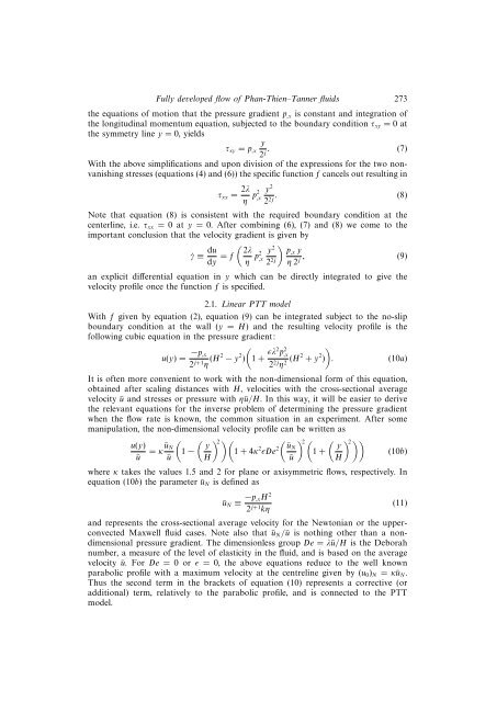
Fully developed flow of Phan-Thien–Tanner fluids 273the equations of motion that the pressure gradient p ,x is constant and integration ofthe longitudinal momentum equation, subjected to the boundary condition τ xy =0atthe symmetry line y = 0, yieldsyτ xy = p ,x2 . (7)jWith the above simplifications and upon division of the expressions for the two nonvanishingstresses (equations (4) and (6)) the specific function f cancels out resulting inτ xx = 2λ y 2η p2 ,x . (8)22j Note that equation (8) is consistent with the required boundary condition at thecenterline, i.e. τ xx =0aty = 0. After combining (6), (7) and (8) we come to theimportant conclusion that the velocity gradient is given by˙γ ≡ du ( ) 2λdy = f y 2 p,x yη p2 ,x2 2j η 2 , (9)jan explicit differential equation in y which can be directly integrated to give thevelocity profile once the function f is specified.2.1. Linear PTT modelWith f given by equation (2), equation (9) can be integrated subject to the no-slipboundary condition at the wall (y = H) and the resulting velocity profile is thefollowing cubic equation in the pressure gradient:()u(y) = −p ,x2 j+1 η (H2 − y 2 )1+ ɛλ2 p 2 ,x2 2j η 2 (H2 + y 2 ). (10a)It is often more convenient to work with the non-dimensional form of this equation,obtained after scaling distances with H, velocities with the cross-sectional averagevelocity ū and stresses or pressure with ηū/H. In this way, it will be easier to derivethe relevant equations for the inverse problem of determining the pressure gradientwhen the flow rate is known, the common situation in an experiment. After somemanipulation, the non-dimensional velocity profile can be written asu(y)ū= κūN ū(1 −( yH) 2 )(1+4κ 2 ɛDe 2 (ūNū) 2 (1+( yH) 2 ))(10b)where κ takes the values 1.5 and 2 for plane or axisymmetric flows, respectively. Inequation (10b) the parameter ū N is defined asū N ≡ −p ,xH 2(11)2 j+1 kηand represents the cross-sectional average velocity for the Newtonian or the upperconvectedMaxwell fluid cases. Note also that ū N /ū is nothing other than a nondimensionalpressure gradient. The dimensionless group De = λū/H is the Deborahnumber, a measure of the level of elasticity in the fluid, and is based on the averagevelocity ū. ForDe =0orɛ = 0, the above equations reduce to the well knownparabolic profile with a maximum velocity at the centreline given by (u 0 ) N = κū N .Thus the second term in the brackets of equation (10) represents a corrective (oradditional) term, relatively to the parabolic profile, and is connected to the PTTmodel.