Distributed Data Mining in Credit Card Fraud Detection

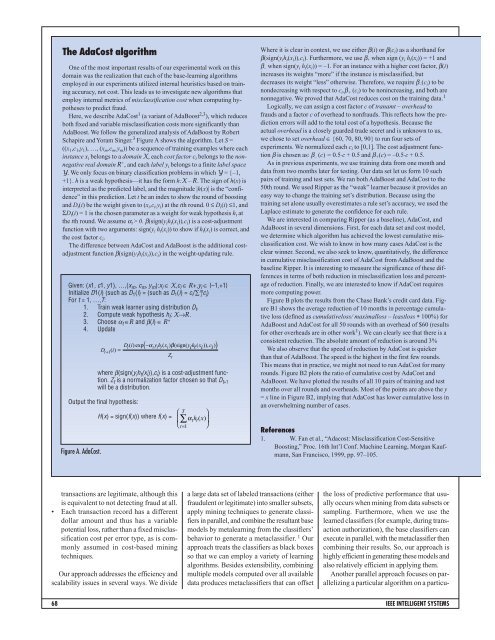
The AdaCost algorithmOne of the most important results of our experimental work on thisdomain was the realization that each of the base-learning algorithmsemployed in our experiments utilized internal heuristics based on trainingaccuracy, not cost. This leads us to investigate new algorithms thatemploy internal metrics of misclassification cost when computing hypothesesto predict fraud.Here, we describe AdaCost 1 (a variant of AdaBoost 2,3 ), which reducesboth fixed and variable misclassification costs more significantly thanAdaBoost. We follow the generalized analysis of AdaBoost by RobertSchapire and Yoram Singer. 3 Figure A shows the algorithm. Let S =((x 1 ,c 1 ,y 1 ), …, (x m ,c m ,y m )) be a sequence of training examples where eachinstance x i belongs to a domain X, each cost factor c i belongs to the nonnegativereal domain R + , and each label y i belongs to a finite label spaceY. We only focus on binary classification problems in which Y = {–1,+1}. h is a weak hypothesis—it has the form h:X – R. The sign of h(x) isinterpreted as the predicted label, and the magnitude |h(x)| is the “confidence”in this prediction. Let t be an index to show the round of boostingand D t (i) be the weight given to (x i ,c i ,y i ) at the tth round. 0 ≤ D t (i) ≤1, andΣD t (i) = 1 is the chosen parameter as a weight for weak hypothesis h t atthe tth round. We assume α t > 0. β(sign(y i h t (x i )),c i ) is a cost-adjustmentfunction with two arguments: sign(y i h t (x i )) to show if h t (x i ) is correct, andthe cost factor c i .The difference between AdaCost and AdaBoost is the additional costadjustmentfunction β(sign(y i h t (x i )),c i ) in the weight-updating rule.Given: (x1, c1, y1), …,(x m , c m , y m ):x i ∈ X,c i ∈ R+,y i ∈ {–1,+1}Initialize D1(i) (such as D 1 (i) = (such as D 1 (i) = c i /∑ m j c j )For t = 1, …,T:1. Train weak learner using distribution D t .2. Compute weak hypothesis h t : X→R.3. Choose α t ∈R and β(i) ∈ R +4. UpdateFigure A. AdaCost.Dt i − tyh i t xiy h x cDtii t i i+ 1 () ( ) exp α ( ) β( sign( ( )), )=Ztwhere β(sign(y i h t (x i )),c i ) is a cost-adjustment function.Z t is a normalization factor chosen so that D t+1will be a distribution.Output the final hypothesis:H(x) = sign(f(x)) where f(x) =( )⎛ T ⎞⎜∑α t h t ( x)⎟⎝ t=1 ⎠Where it is clear in context, we use either β(i) or β(c i ) as a shorthand forβ(sign(y i h t (x i )),c i ). Furthermore, we use β + when sign (y i h t (x i )) = +1 andβ – when sign(y i h t (x i )) = –1. For an instance with a higher cost factor, β(i)increases its weights “more” if the instance is misclassified, butdecreases its weight “less” otherwise. Therefore, we require β – (c i ) to benondecreasing with respect to c i ,β + (c i ) to be nonincreasing, and both arenonnegative. We proved that AdaCost reduces cost on the training data. 1Logically, we can assign a cost factor c of tranamt – overhead tofrauds and a factor c of overhead to nonfrauds. This reflects how the predictionerrors will add to the total cost of a hypothesis. Because theactual overhead is a closely guarded trade secret and is unknown to us,we chose to set overhead ∈ {60, 70, 80, 90} to run four sets ofexperiments. We normalized each c i to [0,1]. The cost adjustment functionβ is chosen as: β – (c) = 0.5⋅c + 0.5 and β + (c) = –0.5⋅c + 0.5.As in previous experiments, we use training data from one month anddata from two months later for testing. Our data set let us form 10 suchpairs of training and test sets. We ran both AdaBoost and AdaCost to the50th round. We used Ripper as the “weak” learner because it provides aneasy way to change the training set’s distribution. Because using thetraining set alone usually overestimates a rule set’s accuracy, we used theLaplace estimate to generate the confidence for each rule.We are interested in comparing Ripper (as a baseline), AdaCost, andAdaBoost in several dimensions. First, for each data set and cost model,we determine which algorithm has achieved the lowest cumulative misclassificationcost. We wish to know in how many cases AdaCost is theclear winner. Second, we also seek to know, quantitatively, the differencein cumulative misclassification cost of AdaCost from AdaBoost and thebaseline Ripper. It is interesting to measure the significance of these differencesin terms of both reduction in misclassification loss and percentageof reduction. Finally, we are interested to know if AdaCost requiresmore computing power.Figure B plots the results from the Chase Bank’s credit card data. FigureB1 shows the average reduction of 10 months in percentage cumulativeloss (defined as cumulativeloss/ maximalloss – leastloss * 100%) forAdaBoost and AdaCost for all 50 rounds with an overhead of $60 (resultsfor other overheads are in other work 1 ). We can clearly see that there is aconsistent reduction. The absolute amount of reduction is around 3%We also observe that the speed of reduction by AdaCost is quickerthan that of AdaBoost. The speed is the highest in the first few rounds.This means that in practice, we might not need to run AdaCost for manyrounds. Figure B2 plots the ratio of cumulative cost by AdaCost andAdaBoost. We have plotted the results of all 10 pairs of training and testmonths over all rounds and overheads. Most of the points are above the y= x line in Figure B2, implying that AdaCost has lower cumulative loss inan overwhelming number of cases.References1. W. Fan et al., “Adacost: Misclassification Cost-SensitiveBoosting,” Proc. 16th Int’l Conf. Machine Learning, Morgan Kaufmann,San Francisco, 1999, pp. 97–105.transactions are legitimate, although thisis equivalent to not detecting fraud at all.• Each transaction record has a differentdollar amount and thus has a variablepotential loss, rather than a fixed misclassificationcost per error type, as is commonlyassumed in cost-based miningtechniques.Our approach addresses the efficiency andscalability issues in several ways. We dividea large data set of labeled transactions (eitherfraudulent or legitimate) into smaller subsets,apply mining techniques to generate classifiersin parallel, and combine the resultant basemodels by metalearning from the classifiers’behavior to generate a metaclassifier. 1 Ourapproach treats the classifiers as black boxesso that we can employ a variety of learningalgorithms. Besides extensibility, combiningmultiple models computed over all availabledata produces metaclassifiers that can offsetthe loss of predictive performance that usuallyoccurs when mining from data subsets orsampling. Furthermore, when we use thelearned classifiers (for example, during transactionauthorization), the base classifiers canexecute in parallel, with the metaclassifier thencombining their results. So, our approach ishighly efficient in generating these models andalso relatively efficient in applying them.Another parallel approach focuses on parallelizinga particular algorithm on a particu-68 IEEE INTELLIGENT SYSTEMS