Methods of Applied Mathematics Lecture Notes

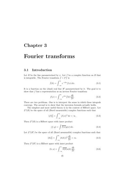
Chapter 3Fourier transforms3.1 IntroductionLet R be the line parameterized by x. Let f be a complex function on R thatis integrable. The Fourier transform ˆf = F f isˆf(k) =∫ ∞−∞e −ikx f(x) dx. (3.1)It is a function on the (dual) real line R ′ parameterized by k. The goal is toshow that f has a representation as an inverse Fourier transformf(x) =∫ ∞−∞e ikx ˆf(k)dk2π . (3.2)There are two problems. One is to interpret the sense in which these integralsconverge. The second is to show that the inversion formula actually holds.The simplest and most useful theory is in the context of Hilbert space. LetL 2 (R) be the space of all (Borel measurable) complex functions such that‖f‖ 2 2 =∫ ∞−∞|f(x)| 2 dx < ∞. (3.3)Then L 2 (R) is a Hilbert space with inner product∫(f, g) = f(x)g(x) dx. (3.4)Let L 2 (R ′ ) be the space of all (Borel measurable) complex functions such that‖h‖ 2 2 =∫ ∞−∞Then L 2 (R ′ ) is a Hilbert space with inner product(h, u) =∫ ∞|h(k))| 2 dk < ∞. (3.5)2π−∞45h(k)u(k) dk2π . (3.6)