LDF Curve-Fitting and Stochastic Reserving: A Maximum Likelihood ...

More documents

Recommendations

Info

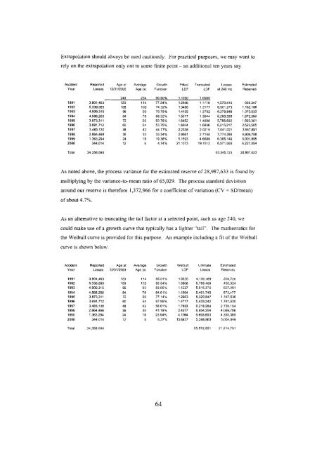
Extrapolation should always be used cautiously. For practical purposes, we may want torely on the extrapolation only out to some finite point - an additional ten years say.Accident Reported Age at Average Growth Fitted Truncated Losses EstimatedYear Losses "i2/3112000 Age (x) Function LDF LDF at 240 mo Reserves240 234 90.50% 1.1050 100001991 3,901,463 120 114 77.24% 1.2946 1.1716 4,570,810 669,3471992 5,339,085 108 192 74.32% 1.3456 1.2177 6,501,273 1,162,1881993 4,909,315 96 90 70.75% 1,4135 1.2792 6,279,848 1,370,5331994 4,588,268 84 78 66.32% 15077 13644 6,260,356 1,672,0901995 3,873,311 72 66 6078% 1.6452 1.4888 5,766,692 1,893,3811996 3,691,712 60 54 5375% 1.8604 1.6836 6,215,217 2,523,5951997 3,483,130 48 42 44,77% 2.2338 2,0215 7,041,021 3,557,8911998 2,864,498 36 30 3334% 29991 27140 7,774,286 4,909,7881999 1,363,294 24 18 19 38% 5.1593 4.6689 6,365,149 5,001,8552000 344,014 12 6 4.74% 21.1073 191012 6,571,068 6.227,054Total 34,358,090 83,345,723 28.987,633As noted above, the process variance for the estimated reserve of 28,987,633 is found bymultiplying by the variance-to-mean ratio of 65,029. The process standard deviationaround our reserve is therefore 1,372,966 for a coefficient of variation (C V = SD/mean)of about 4.7%.As an alternative to truncating the tail factor at a selected point, such as age 240, wecould make use of a growth curve that typically has a lighter "tail". The mathematics forthe WeibuIl curve is provided for this purpose. An example including a fit of the Weibullcurve is shown below.Accident Reported Age at Average Growth WeibuEI Uitlmate EstimatedYear Losses 12/31/2000 Age (x) Function LDF Losses Reserves1991 3,901,463 120 114 95.91% 1,0525 4,106,189 204,7261992 5,339,085 108 102 9254% 1,0806 5,769,409 430,3241993 4,909,315 96 90 89.00% 1.1237 5,516,376 807,0611994 4,888,268 84 78 84.01% 1.1904 5,461,745 873,4771995 3,873,311 72 66 7714% 1.2963 5,020,847 1,147,5361996 3,691,712 60 54 6795% 1.4717 5,433,242 1,741,5301997 3,483,136 48 42 5601% 1.7853 6,218,284 2,735,1541998 2,864,498 36 30 41.19% 2.4277 6,954,204 4,089,7061999 1,363,294 24 18 23.94% 41764 5,693,693 4,330,3992000 344,014 12 6 6.37% 15.6937 5,398,863 5,054,849Total 34,358,090 55,572,851 21,214,76164
The fitted Weibull parameters 0 and to are 48.88453 and 1.296906, respectively. Thelower "tail" factor of 1.0525 (instead of 1.2946 for the Loglogistic) may be more in linewith the actuary's expectation for casualty business. The difference between the twocurve forms also highlights the danger in relying on a purely mechanical extrapolationformula. The selection of a truncation point is an effective way of reducing the relianceon the extrapolation when the thicker-tailed Loglogistic is used.The next step is our estimate of the parameter variance.The parameter variance calculation is more involved than what was needed for processvariance. As discussed in Section 2.3, we need to first evaluate the Information Matrix,which contains the second derivatives with respect to all of the model parameters, and sois a 12x12 matrix. The mathematics for all of these calculations is given in Appendix A,and is not difficult to program in most sottware. For purposes of this example, we willsimply show the resulting variances:Accident Reported Estimated Process Parameter TotalYear Losses Resen,~ Std Dev CV Std Dev CV Std Dev CV1991 3,901,463 669,347 208,631 31.2% 158,088 23.6% 261,761 39.1%1992 5,339,085 1,162,188 274,911 23.7% 257,205 22.1% 376,471 32.4%1993 4,909,315 1,370,533 298,537 21.8% 298,628 21.8% 422,260 30.8%1994 4,588,268 1,672,090 329,749 19.7% 356.827 21.3% 485,860 29.1%1995 3,873,311 1,893,381 350,891 18.5% 401,416 21.2% 533,160 28.2%1996 3,691.712 2,523,505 405,(F34 16.1% 518,226 20.5% 657,768 26.1%1997 3,483,130 3,557,891 481,005 13.5% 704,523 19.8% 853,064 24.0%1998 2.864,498 4,909,788 565,047 11.5% 968,806 19.7% 1,121,545 22.8%1999 1,363.294 5,001,855 570,321 11.4% 1,227,880 24.5% 1.353.867 27.1%2000 344,014 6,227,054 636,348 10.2% 2,838,890 45.6% 2,909,336 46.7%Total 34,358,090 28,987,633 1,372,966 4.7% 4,688,826 16.2% 4,885,707 16.9%From this table, one conclusion should be readily apparent: the parameter variancecomponent is much more significant than the process variance. The chief reason for thisis that we have overparameterization of our model; that is, the available 55 data points arereally not sufficient-to estimate the 12 parameters of the model. The 1994 Zehnwirthpaper ([ 10], p. 512t) gives a helpful discussion of the dangers of overparameterization.65
Page 1 and 2: LDF Curve-Fitting and Stochastic Re
Page 3 and 4: IntroductionMany papers have been w
Page 5 and 6: Section 1:Expected Loss EmergenceOu
Page 7 and 8: amonnt in each accident year is ind
Page 9 and 10: Section 2:The Distribution of Actua
Page 11 and 12: This can be maximized using the log
Page 13 and 14: 2.3 Parameter Variance 6The second
Page 15 and 16: lThe future reserve R, under the Ca
Page 17 and 18: Unfortunately, including the scale
Page 19 and 20: Section 4:A Practical Example4.1 Th
Page 21 and 22: - producingages 12, 24, 36, etc - b
Page 23: ¢l -!321_~ 0i -1 -2z -34 .........
Page 27 and 28: For the example in the Mack paper,
Page 29 and 30: the 65,029 calculated for the LDF m
Page 31 and 32: 4.3.2 Calendar Year DevelopmentThe
Page 33 and 34: Section 5: Comments and Conclusion5
Page 35 and 36: The chief result that we observe in
Page 37 and 38: Table 1.2Triangle Collapsed for Lat
Page 39 and 40: Table 1.4Original Triangle along wi
Page 41 and 42: References:[ 1 ] England & Verrall;
Page 43 and 44: ~2e3co 30_- y_I[ -~,, ,IP ~(x,) ~u,
Page 45 and 46: Loglogistic Distribution (for "inve
Page 47 and 48: 1) Calculate the percent of the per
Page 49 and 50: Appendix C: Variance in Discounted
Page 51: In order to calculate the derivativ

LDF Curve-Fitting and Stochastic Reserving: A Maximum Likelihood ...

Create successful ePaper yourself

Delete template?

Save as template?