Phase shifts between synchronized oscillators in the Winfree and ...

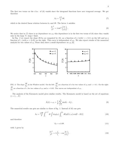
The first two terms on the r.h.s. of (6) vanish since the integrand functions have zero temporal average. We gettherefore3δω = κλ 2δθ, (7)which is the desired linear relation between δω and δθ. The factor λ satisfies4γ 2 ( ) 2γκ 2 = λ sin2 . (8)κλWe notice that in (7) there is no dependence on ω 0 ; this dependence is in the first two terms of (6) since they vanishonly in the large N, large t limit.In Fig. 2 we report the slope δθ/δω as computed by (8), as a function of κ (with γ = 0.1) on the left and as afunction of γ (with κ = 0.45) on the right. This curve is independent of ω 0 . We also report results of the numericalanalysis for two values of ω 0 These data show a small dependence on ω 0 [6].108Ω 0 ⩵ 1Ω 0 ⩵ 2108Ω 0 ⩵ 1Ω 0 ⩵ 2∆Θ∆Ω64∆Θ∆Ω64220.3 0.4 0.5 0.6 0.7Κ0 0.02 0.04 0.06 0.08 0.1 0.12ΓFIG. 2: The slope δθδω in the Winfree model. On the left: δθas a function of κ for two values of ω0 and γ = 0.1. On the right:δωδθas a function of γ for two values of ω0 and κ = 0.45. The curves are independent of ω0.δωThe analysis of the Kuramoto model gives similar results. The Kuramoto model is based on the set of equations(i = 1, ...N)˙θ i (t) = ω i + κ NN∑sin(θ i − θ j ) . (9)j=1The numerical results one gets are similar to those of fig. 1. Instead of (6) one getsand thereforeδω = κδθT∫ t+Tt∫dtdωg(ω)∫ 2π0dˆθ p(ˆθ, t, ω) cos[ˆθ − θ(t)] (10)δω = κλ δθ . (11)with λ given by2γ 2 (κ 2 = λ 1 − cos 2γ ). (12)κλ