Modeling of optimal perturbations in flat plate boundary ... - Ensam

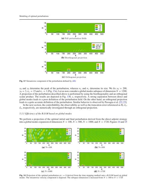
Modeling of optimal perturbations(a)(b)Fig. 13 Streamwise component of the perturbation defined by (40)(c)x 0 and y 0 determine the peak of the perturbation, whereas σ x and σ y determine its size. We fix x 0 = 200,y 0 = 3, σ x = 15 and σ y = 1(Fig.13a). Let us now consider a global modes subspace of dimension N = 1200.A projection of the perturbation described above is performed by using the biorthogonality and an orthogonalscalar product. The results are depicted in Fig. 13b, c, respectively. A strong separation between direct andglobal modes leads to a poor definition of the perturbation field. On the other hand, an orthogonal projectionleads to a quite accurate definition of the perturbation. Similar behavior is observed by Passagia et al. [22,23].In the next section, the controllability, the observability as well as the truncation error referenced as B k C k ,E k , respectively, are numerically investigated through an orthogonal projection.5.3.3 Efficiency of the R.O.M based on global modesWe perform a projection of the optimal initial and final perturbation derived from the direct-adjoint strategyinto a global modes expansion of dimension N = 100, N = 500, N = 1000, and N = 1720. Figures 14 and 15(a)(b)(c)Fig. 14 Projection of the optimal perturbation at t = 0 derived from the time-stepping method onto a R.O.M based on globalmodes. The streamwise velocity component is depicted. The subspace dimension is increased from N = 100 to N = 1720(d)