The nonequilibrium thermodynamics of small systems

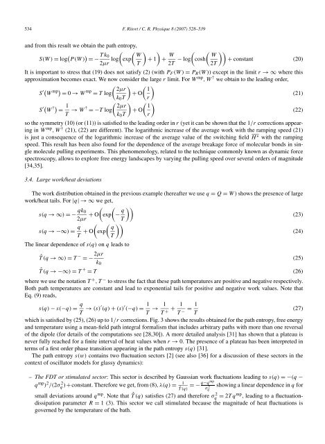
534 F. Ritort / C. R. Physique 8 (2007) 528–539and from this result we obtain the path entropy,S(W) = log ( P(W) ) =− Tk ( ( ) )0 W2μr log exp + 1 + W ( ( )) WT 2T − log cosh + constant (20)2TIt is important to stress that (19) does not satisfy (2) (with P F (W ) = P R (W )) except in the limit r →∞where thisapproximation becomes exact. We now consider the large r limit. For W mp ,W † we obtain to the leading order,S ′( W mp) ( ) ( )2μr 1= 0 → W mp = T log + O(21)k 0 T rS ′( W †) = 1 ( ) ( )2μr 1T → W † =−T log + O(22)k 0 T rso the symmetry (10) (or (11)) is satisfied to the leading order in r (yet it can be shown that the 1/r corrections appearingin W mp ,W † (21), (22) are different). The logarithmic increase of the average work with the ramping speed (21)is just a consequence of the logarithmic increase of the average value of the switching field H ∗ with the rampingspeed. This result has been also found for the dependence of the average breakage force of molecular bonds in singlemolecule pulling experiments. This phenomenology, related to the technique commonly known as dynamic forcespectroscopy, allows to explore free energy landscapes by varying the pulling speed over several orders of magnitude[34,35].3.4. Large work/heat deviationsThe work distribution obtained in the previous example (hereafter we use q = Q = W ) shows the presence of largework/heat tails. For |q|→∞we get,s(q →∞) =− qk ( (02μr + O exp − q ))(23)Ts(q →−∞) = q ( )) q(expT + O (24)TThe linear dependence of s(q) on q leads toˆT(q→∞) = T − =− 2μr(25)k 0ˆT(q→−∞) = T + = T (26)where we use the notation T + ,T − to stress the fact that these path temperatures are positive and negative respectively.Both path temperatures are constant and lead to exponential tails for positive and negative work values. Note thatEq. (9) reads,s(q) − s(−q) = q T → (s)′ (q) + (s) ′ (−q) = 1 T → 1T + + 1T − = 1 (27)Twhich is satisfied by (25), (26) up to 1/r corrections. Fig. 3 shows the results obtained for the path entropy, free energyand temperature using a mean-field path integral formalism that includes arbitrary paths with more than one reversalof the dipole (for details of the computations see [28,30]). A more detailed analysis [31] has shown that a plateau isnever fully reached for a finite interval of heat values when r → 0. The presence of a plateau has been interpreted interms of a first order phase transition appearing in the path entropy s(q) [31].The path entropy s(w) contains two fluctuation sectors [2] (see also [36] for a discussion of these sectors in thecontext of oscillator models for glassy dynamics):– The FDT or stimulated sector: This sector is described by Gaussian work fluctuations leading to s(q) =−(q −q mp ) 2 /(2σq 2 1)+constant. Therefore we get, from (8), λ(q) =ˆT(q) =−q−qmp showing a linear dependence in q forσq2small deviations around q mp . Note that ˆT(q) satisfies (27) and therefore σq 2 = 2Tqmp , leading to a fluctuationdissipationparameter R = 1 (3). This sector we call stimulated because the magnitude of heat fluctuations isgoverned by the temperature of the bath.