Efficient Portfolio Optimization with Conditional Value at Risk

More documents

Recommendations

Info

904 PROCEEDINGS OF THE IMCSIT. VOLUME 5, 2010with the inner optimization problemD(u) = maxx j{T∑ ∑nu t r jt x j :t=1j=1n∑µ j x j ≥ µ 0 ,j=1n∑x j = 1,j=1x j ≥ 0, j = 1,...,n}n∑ T∑= max { ( r jt u t )x j :x jj=1t=1n∑µ j x j ≥ µ 0 ,j=1n∑x j = 1,j=1x j ≥ 0, j = 1,...,n}.(11)Again, we may take advantages of the LP dual to the innerproblem. Indeed, introducing dual variable q corresponding tothe equation ∑ nj=1 x j = 1 and variable u 0 corresponding tothe inequality ∑ nj=1 µ jx j ≥ µ 0 we get the LP dualD(u) = minq,u 0{q −µ 0 u 0 :q −µ j u 0 −T∑r jt u t ≥ 0 j = 1,...,n}.t=1Hence, an alternative model for the CVaR portfolio optimization(10) can be expressed as the following LP:min q −µ 0 u 0s.t. q −µ j u 0 −T∑r jt u t ≥ 0, j = 1,...,nt=1T∑(12)u t = 1t=10 ≤ u t ≤ p tβ , t = 1,...,TLP model (12) contains T + 1 variables u t , but the Tconstraints corresponding to variables d t from (6) take theform of simple upper bounds on u t (for t = 1,...,T)thus not affecting the problem complexity. The number ofconstraints in (12) is proportional to the total of portfoliosize n, thus it is independent from the number of scenarios.Exactly, there are T +1 variables and n+1 constraints. Thisguarantees a high computational efficiency of the model evenfor very large number of scenarios. Similarly, other portfoliostructure requirements are modeled with rather small numberof constraints thus generating small number of additionalvariables in the model. Actually, the model (12) is the LPdual to the model (6), thus similar to that introduced in [23].Obviously, the optimal portfolio shares x j are not directlyrepresentedwithinthe solutionvectorofproblem(12)buttheyare easily available as the dual variables (shadow prices) forinequalities q −µ j u 0 − ∑ Tt=1 r jtu t ≥ 0.The Minimax portfolio optimization model can be writtenas the following LP problem:max ηn∑s.t. µ j x j ≥ µ 0 ,j=1n∑x j = 1j=1x j ≥ 0, j = 1,...,nn∑−η + r jt x j ≥ 0, t = 1,...,Tj=1(13)which is simpler than the standard CVaR optimization model(6). Except from the portfolio weights x j , the model containsonly one additional variable η. Nevertheless, it still contains Tlinear inequalities in addition to the core constraints. Hence,its dimensionality is (T +2)×(n+1).The Minimax portfolio optimization model representing alimiting case of the CVaR model for β tending to 0. Actually,for any β ≤ min t=1,...,T p t we gets M β (x) = M(x) thusallowing to represent the Minimax portfolio optimization bythe CVaR optimization model (6) and to take advantagesof itsdual form (12). Due to β ≤ p t for all t = 1,...,T, the upperbounds on variables u t becomes redundant and we get thefollowing dual form of the Minimax portfolio optimization:min q −µ 0 u 0s.t. q −µ j u 0 −T∑u t = 1t=1T∑r jt u t ≥ 0, j = 1,...,nt=1u t ≥ 0, t = 1,...,T(14)The model dimensionality is only (n + 1) × (T + 2) thusguaranteeing a high computational efficiency even for verylarge number of scenarios.The Mean Absolute Deviation (MAD) risk measure isdirectly given by the value of the second order cdf F x(2) atthe mean ¯δ(x) = E{max{µ(x)−R x ,0}} = F x (2) (µ(x)) [19].Therefore,its leadstoan LP portfoliooptimizationmodelverysimilar to that for the CVaR optimization (6). Indeed, we get:max −s.t.T∑p t d tt=1n∑µ j x j ≥ µ 0 ,j=1d t ≥n∑x j = 1j=1n∑(µ j −r jt )x j , d t ≥ 0, t = 1,...,Tj=1x j ≥ 0, j = 1,...,n(15)with T+n variablesand T+2 constraints. The LP dual model
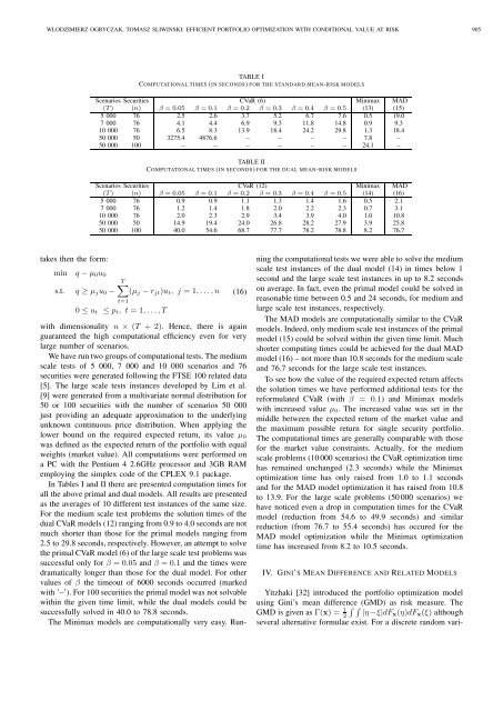
WLODZIMIERZ OGRYCZAK, TOMASZ SLIWINSKI: EFFICIENT PORTFOLIO OPTIMIZATION WITH CONDITIONAL VALUE AT RISK 905TABLE ICOMPUTATIONAL TIMES (IN SECONDS) FOR THE STANDARD MEAN-RISK MODELSScenarios Securities CVaR (6) Minimax MAD(T) (n) β = 0.05 β = 0.1 β = 0.2 β = 0.3 β = 0.4 β = 0.5 (13) (15)5 000 76 2.5 2.6 3.7 5.2 6.7 7.6 0.5 19.07 000 76 4.1 4.4 6.9 9.3 11.8 14.8 0.9 9.310 000 76 6.5 8.3 13.9 18.4 24.2 29.8 1.3 18.450 000 50 3275.4 4876.6 – – – – 7.8 –50 000 100 – – – – – – 24.1 –TABLE IICOMPUTATIONAL TIMES (IN SECONDS) FOR THE DUAL MEAN-RISK MODELSScenarios Securities CVaR (12) Minimax MAD(T) (n) β = 0.05 β = 0.1 β = 0.2 β = 0.3 β = 0.4 β = 0.5 (14) (16)5 000 76 0.9 0.9 1.1 1.3 1.4 1.6 0.5 2.17 000 76 1.2 1.4 1.8 2.0 2.2 2.3 0.7 3.110 000 76 2.0 2.3 2.9 3.4 3.9 4.0 1.0 10.850 000 50 14.9 19.4 24.0 26.8 28.2 27.9 3.9 25.850 000 100 40.0 54.6 68.7 77.7 78.2 78.8 8.2 76.7takes then the form:min q −µ 0 u 0s.t. q ≥ µ j u 0 −T∑(µ j −r jt )u t , j = 1,...,nt=10 ≤ u t ≤ p t , t = 1,...,T(16)with dimensionality n × (T + 2). Hence, there is againguaranteed the high computational efficiency even for verylarge number of scenarios.Wehaveruntwogroupsofcomputationaltests.Themediumscale tests of 5 000, 7 000 and 10 000 scenarios and 76securities were generated following the FTSE 100 related data[5]. The large scale tests instances developed by Lim et al.[9] were generated from a multivariate normal distribution for50 or 100 securities with the number of scenarios 50 000just providing an adequate approximation to the underlyingunknown continuous price distribution. When applying thelower bound on the required expected return, its value µ 0was defined as the expected return of the portfolio with equalweights (market value). All computations were performed ona PC with the Pentium 4 2.6GHz processor and 3GB RAMemploying the simplex code of the CPLEX 9.1 package.In Tables I and II there are presented computation times forall the above primal and dual models. All results are presentedas the averages of 10 different test instances of the same size.For the medium scale test problems the solution times of thedualCVaRmodels(12)rangingfrom0.9to4.0secondsarenotmuch shorter than those for the primal models ranging from2.5 to 29.8seconds, respectively.However,an attempt to solvetheprimalCVaRmodel(6)ofthelargescaletestproblemswassuccessful only for β = 0.05 and β = 0.1 and the times weredramatically longer than those for the dual model. For othervalues of β the timeout of 6000 seconds occurred (markedwith ’–’).For 100securitiesthe primalmodelwasnot solvablewithin the given time limit, while the dual models could besuccessfully solved in 40.0 to 78.8 seconds.The Minimax models are computationally very easy. Runningthecomputationaltestswe were ableto solvethe mediumscale test instances of the dual model (14) in times below 1second and the large scale test instances in up to 8.2 secondson average. In fact, even the primal model could be solved inreasonable time between 0.5 and 24 seconds, for medium andlarge scale test instances, respectively.The MAD models are computationally similar to the CVaRmodels.Indeed,onlymediumscale test instancesofthe primalmodel (15) could be solved within the given time limit. Muchshorter computing times could be achieved for the dual MADmodel(16)– not morethan 10.8secondsfor the mediumscaleand 76.7 seconds for the large scale test instances.To see how the value of the required expected return affectsthe solution times we have performed additional tests for thereformulated CVaR (with β = 0.1) and Minimax modelswith increased value µ 0 . The increased value was set in themiddle between the expected return of the market value andthe maximum possible return for single security portfolio.The computational times are generally comparable with thosefor the market value constraints. Actually, for the mediumscale problems (10000 scenarios) the CVaR optimization timehas remained unchanged (2.3 seconds) while the Minimaxoptimization time has only raised from 1.0 to 1.1 secondsand for the MAD model optimization it has raised from 10.8to 13.9. For the large scale problems (50000 scenarios) wehave noticed even a drop in computation times for the CVaRmodel (reduction from 54.6 to 49.9 seconds) and similarreduction (from 76.7 to 55.4 seconds) has occured for theMAD model optimization while the Minimax optimizationtime has increased from 8.2 to 10.5 seconds.IV. GINI’S MEAN DIFFERENCE AND RELATED MODELSYitzhaki [32] introduced the portfolio optimization modelusing Gini’s mean difference ∫ ∫ (GMD) as risk measure. TheGMD is given as Γ(x) = 1 2 |η−ξ|dFx (η)dF x (ξ) althoughseveral alternative formulae exist. For a discrete random vari-
Page 6 and 7: 906 PROCEEDINGS OF THE IMCSIT. VOLU
Page 8: 908 PROCEEDINGS OF THE IMCSIT. VOLU

Efficient Portfolio Optimization with Conditional Value at Risk

You also want an ePaper? Increase the reach of your titles

Delete template?

Save as template?