- Page 1 and 2: . Chaos: Classical and QuantumI: De
- Page 3 and 4: CONTENTSiii5.3 Stability of Poincar
- Page 5 and 6: CONTENTSv18 Cycle expansions 29918.
- Page 7 and 8: CONTENTSviiPart II: Quantum chaos29
- Page 9 and 10: CONTENTSixPart III: Appendices on C
- Page 11 and 12: CONTENTSxiContributorsNo man but a
- Page 13: CONTENTSxiii4.5.1 Stability of Poin
- Page 16 and 17: Chapter 1OvertureIf I have seen les
- Page 18 and 19: CHAPTER 1. OVERTURE 3this material,
- Page 20 and 21: CHAPTER 1. OVERTURE 5231323212Figur
- Page 22 and 23: CHAPTER 1. OVERTURE 7Figure 1.4: Dy
- Page 24 and 25: CHAPTER 1. OVERTURE 9Figure 1.5: Ka
- Page 26 and 27: CHAPTER 1. OVERTURE 11Figure 1.7: T
- Page 28 and 29: CHAPTER 1. OVERTURE 13of survivors
- Page 30 and 31: CHAPTER 1. OVERTURE 15where Λ i is
- Page 32 and 33: CHAPTER 1. OVERTURE 171.5.3 Cycle e
- Page 34 and 35: CHAPTER 1. OVERTURE 191.6 Evolution
- Page 36 and 37: CHAPTER 1. OVERTURE 21The beauty of
- Page 38 and 39: CHAPTER 1. OVERTURE 23So, no proofs
- Page 40 and 41: CHAPTER 1. OVERTURE 25But the power
- Page 42 and 43: CHAPTER 1. OVERTURE 27measures of
- Page 44 and 45: EXERCISES 29Exercises1.1. 3-disk sy
- Page 46 and 47: References 31[1.29] D. Ruelle, “F
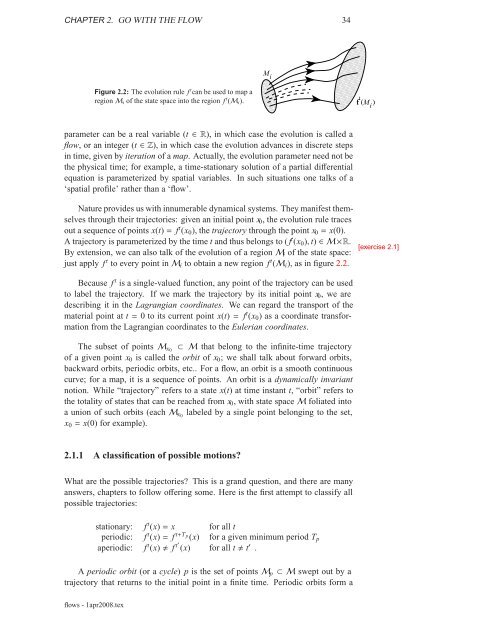
- Page 50 and 51: CHAPTER 2. GO WITH THE FLOW 35very
- Page 52 and 53: CHAPTER 2. GO WITH THE FLOW 37asymp
- Page 54 and 55: CHAPTER 2. GO WITH THE FLOW 39Z(t)3
- Page 56 and 57: CHAPTER 2. GO WITH THE FLOW 41some
- Page 58 and 59: EXERCISES 43The exercises that you
- Page 60 and 61: References 45[2.7] D. Rothman, Nonl
- Page 62 and 63: CHAPTER 3. DISCRETE TIME DYNAMICS 4
- Page 64 and 65: CHAPTER 3. DISCRETE TIME DYNAMICS 4
- Page 66 and 67: CHAPTER 3. DISCRETE TIME DYNAMICS 5
- Page 68 and 69: CHAPTER 3. DISCRETE TIME DYNAMICS 5
- Page 70 and 71: CHAPTER 3. DISCRETE TIME DYNAMICS 5
- Page 72 and 73: CHAPTER 3. DISCRETE TIME DYNAMICS 5
- Page 74 and 75: EXERCISES 59Exercises3.1. Poincaré
- Page 76 and 77: Chapter 4Local stability(R. Mainier
- Page 78 and 79: CHAPTER 4. LOCAL STABILITY 63x(t)δ
- Page 80 and 81: CHAPTER 4. LOCAL STABILITY 65Hence
- Page 82 and 83: CHAPTER 4. LOCAL STABILITY 67Exampl
- Page 84 and 85: CHAPTER 4. LOCAL STABILITY 69are fl
- Page 86 and 87: CHAPTER 4. LOCAL STABILITY 714.3 St
- Page 88 and 89: CHAPTER 4. LOCAL STABILITY 73Figure
- Page 90 and 91: CHAPTER 4. LOCAL STABILITY 75task a
- Page 92 and 93: CHAPTER 4. LOCAL STABILITY 77hand s
- Page 94 and 95: CHAPTER 4. LOCAL STABILITY 79Figure
- Page 96 and 97: EXERCISES 81The nomenclature tends
- Page 98 and 99:
Chapter 5Cycle stabilityTopological
- Page 100 and 101:
CHAPTER 5. CYCLE STABILITY 85Figure
- Page 102 and 103:
CHAPTER 5. CYCLE STABILITY 87Exampl
- Page 104 and 105:
CHAPTER 5. CYCLE STABILITY 89so a p
- Page 106 and 107:
EXERCISES 91infinite set of metric
- Page 108 and 109:
Chapter 6Get straightWe owe it to a
- Page 110 and 111:
CHAPTER 6. GET STRAIGHT 95smoothly,
- Page 112 and 113:
CHAPTER 6. GET STRAIGHT 97Figure 6.
- Page 114 and 115:
CHAPTER 6. GET STRAIGHT 99Example 6
- Page 116 and 117:
CHAPTER 6. GET STRAIGHT 1016.4 Rect
- Page 118 and 119:
CHAPTER 6. GET STRAIGHT 1036.6 Cycl
- Page 120 and 121:
CHAPTER 6. GET STRAIGHT 105Remark 6
- Page 122 and 123:
References 107[6.10] I. Percival an
- Page 124 and 125:
CHAPTER 7. HAMILTONIAN DYNAMICS 109
- Page 126 and 127:
CHAPTER 7. HAMILTONIAN DYNAMICS 111
- Page 128 and 129:
CHAPTER 7. HAMILTONIAN DYNAMICS 113
- Page 130 and 131:
CHAPTER 7. HAMILTONIAN DYNAMICS 115
- Page 132 and 133:
EXERCISES 117Put your right hand on
- Page 134 and 135:
References 119[7.5] D.G. Sterling,
- Page 136 and 137:
CHAPTER 8. BILLIARDS 121Figure 8.1:
- Page 138 and 139:
CHAPTER 8. BILLIARDS 123Consider a
- Page 140 and 141:
EXERCISES 125CommentaryRemark 8.1 B
- Page 142 and 143:
References 127[8.7] G. Vattay, A. W
- Page 144 and 145:
CHAPTER 9. WORLD IN A MIRROR 1299.1
- Page 146 and 147:
CHAPTER 9. WORLD IN A MIRROR 1319.1
- Page 148 and 149:
CHAPTER 9. WORLD IN A MIRROR 133{0}
- Page 150 and 151:
CHAPTER 9. WORLD IN A MIRROR 135Fig
- Page 152 and 153:
CHAPTER 9. WORLD IN A MIRROR 137Fig
- Page 154 and 155:
CHAPTER 9. WORLD IN A MIRROR 139Fig
- Page 156 and 157:
CHAPTER 9. WORLD IN A MIRROR 141the
- Page 158 and 159:
CHAPTER 9. WORLD IN A MIRROR 143Exa
- Page 160 and 161:
CHAPTER 9. WORLD IN A MIRROR 145(1)
- Page 162 and 163:
EXERCISES 147Exercises9.1. 3-disk f
- Page 164 and 165:
REFERENCES 1499.9. Proto-Lorenz sys
- Page 166 and 167:
References 151[9.28] R. Miranda and
- Page 168 and 169:
CHAPTER 10. QUALITATIVE DYNAMICS, F
- Page 170 and 171:
CHAPTER 10. QUALITATIVE DYNAMICS, F
- Page 172 and 173:
CHAPTER 10. QUALITATIVE DYNAMICS, F
- Page 174 and 175:
CHAPTER 10. QUALITATIVE DYNAMICS, F
- Page 176 and 177:
CHAPTER 10. QUALITATIVE DYNAMICS, F
- Page 178 and 179:
CHAPTER 10. QUALITATIVE DYNAMICS, F
- Page 180 and 181:
CHAPTER 10. QUALITATIVE DYNAMICS, F
- Page 182 and 183:
CHAPTER 10. QUALITATIVE DYNAMICS, F
- Page 184 and 185:
CHAPTER 10. QUALITATIVE DYNAMICS, F
- Page 186 and 187:
EXERCISES 171Remark 10.2 Counting p
- Page 188 and 189:
References 173[10.10] A. Boyarski,
- Page 190 and 191:
CHAPTER 11. QUALITATIVE DYNAMICS, F
- Page 192 and 193:
CHAPTER 11. QUALITATIVE DYNAMICS, F
- Page 194 and 195:
CHAPTER 11. QUALITATIVE DYNAMICS, F
- Page 196 and 197:
CHAPTER 11. QUALITATIVE DYNAMICS, F
- Page 198 and 199:
CHAPTER 11. QUALITATIVE DYNAMICS, F
- Page 200 and 201:
CHAPTER 11. QUALITATIVE DYNAMICS, F
- Page 202 and 203:
CHAPTER 11. QUALITATIVE DYNAMICS, F
- Page 204 and 205:
CHAPTER 11. QUALITATIVE DYNAMICS, F
- Page 206 and 207:
REFERENCES 191(a) (easy) Consider a
- Page 208 and 209:
References 193[11.26] K.T. Hansen,
- Page 210 and 211:
Chapter 12Fixed points, and how to
- Page 212 and 213:
CHAPTER 12. FIXED POINTS, AND HOW T
- Page 214 and 215:
CHAPTER 12. FIXED POINTS, AND HOW T
- Page 216 and 217:
CHAPTER 12. FIXED POINTS, AND HOW T
- Page 218 and 219:
CHAPTER 12. FIXED POINTS, AND HOW T
- Page 220 and 221:
CHAPTER 12. FIXED POINTS, AND HOW T
- Page 222 and 223:
CHAPTER 12. FIXED POINTS, AND HOW T
- Page 224 and 225:
EXERCISES 209Exercises12.1. Cycles
- Page 226 and 227:
References 211[12.11] B. Doyon and
- Page 228 and 229:
CHAPTER 13. COUNTING 2133e n ln 2
- Page 230 and 231:
CHAPTER 13. COUNTING 21513.2 Topolo
- Page 232 and 233:
CHAPTER 13. COUNTING 217We could no
- Page 234 and 235:
CHAPTER 13. COUNTING 219Figure 13.1
- Page 236 and 237:
CHAPTER 13. COUNTING 221terms of cy
- Page 238 and 239:
CHAPTER 13. COUNTING 223Example 13.
- Page 240 and 241:
Table 13.3: List of the 3-disk prim
- Page 242 and 243:
CHAPTER 13. COUNTING 227Figure 13.4
- Page 244 and 245:
CHAPTER 13. COUNTING 229step in der
- Page 246 and 247:
EXERCISES 231the corresponding tran
- Page 248 and 249:
REFERENCES 233As the rule does not
- Page 250 and 251:
Chapter 14Transporting densitiesPau
- Page 252 and 253:
CHAPTER 14. TRANSPORTING DENSITIES
- Page 254 and 255:
CHAPTER 14. TRANSPORTING DENSITIES
- Page 256 and 257:
CHAPTER 14. TRANSPORTING DENSITIES
- Page 258 and 259:
CHAPTER 14. TRANSPORTING DENSITIES
- Page 260 and 261:
CHAPTER 14. TRANSPORTING DENSITIES
- Page 262 and 263:
CHAPTER 14. TRANSPORTING DENSITIES
- Page 264 and 265:
CHAPTER 14. TRANSPORTING DENSITIES
- Page 266 and 267:
EXERCISES 251quence of Gaussians∫
- Page 268 and 269:
References 253[14.13] G. Froyland,
- Page 270 and 271:
CHAPTER 15. AVERAGING 25515.1.1 Tim
- Page 272 and 273:
CHAPTER 15. AVERAGING 257of the dyn
- Page 274 and 275:
CHAPTER 15. AVERAGING 259so if we c
- Page 276 and 277:
CHAPTER 15. AVERAGING 261Figure 15.
- Page 278 and 279:
CHAPTER 15. AVERAGING 263δx0x(0)δ
- Page 280 and 281:
CHAPTER 15. AVERAGING 265Figure 15.
- Page 282 and 283:
CHAPTER 15. AVERAGING 267Here we ha
- Page 284 and 285:
REFERENCES 26915.1. How unstable is
- Page 286 and 287:
Chapter 16Trace formulasThe trace f
- Page 288 and 289:
CHAPTER 16. TRACE FORMULAS 273magni
- Page 290 and 291:
CHAPTER 16. TRACE FORMULAS 275This
- Page 292 and 293:
CHAPTER 16. TRACE FORMULAS 277be th
- Page 294 and 295:
CHAPTER 16. TRACE FORMULAS 279the f
- Page 296 and 297:
EXERCISES 281Now that we have a tra
- Page 298 and 299:
Chapter 17Spectral determinants“I
- Page 300 and 301:
CHAPTER 17. SPECTRAL DETERMINANTS 2
- Page 302 and 303:
CHAPTER 17. SPECTRAL DETERMINANTS 2
- Page 304 and 305:
CHAPTER 17. SPECTRAL DETERMINANTS 2
- Page 306 and 307:
CHAPTER 17. SPECTRAL DETERMINANTS 2
- Page 308 and 309:
CHAPTER 17. SPECTRAL DETERMINANTS 2
- Page 310 and 311:
CHAPTER 17. SPECTRAL DETERMINANTS 2
- Page 312 and 313:
REFERENCES 297(d) Let p be all prim
- Page 314 and 315:
Chapter 18Cycle expansionsRecycle..
- Page 316 and 317:
CHAPTER 18. CYCLE EXPANSIONS 301We
- Page 318 and 319:
CHAPTER 18. CYCLE EXPANSIONS 303For
- Page 320 and 321:
CHAPTER 18. CYCLE EXPANSIONS 305Giv
- Page 322 and 323:
CHAPTER 18. CYCLE EXPANSIONS 307and
- Page 324 and 325:
CHAPTER 18. CYCLE EXPANSIONS 30918.
- Page 326 and 327:
CHAPTER 18. CYCLE EXPANSIONS 311whi
- Page 328 and 329:
CHAPTER 18. CYCLE EXPANSIONS 313Fig
- Page 330 and 331:
CHAPTER 18. CYCLE EXPANSIONS 315fea
- Page 332 and 333:
EXERCISES 317Exercises18.1. Cycle e
- Page 334 and 335:
REFERENCES 31918.12. Ulam map is co
- Page 336 and 337:
CHAPTER 19. DISCRETE FACTORIZATION
- Page 338 and 339:
CHAPTER 19. DISCRETE FACTORIZATION
- Page 340 and 341:
CHAPTER 19. DISCRETE FACTORIZATION
- Page 342 and 343:
CHAPTER 19. DISCRETE FACTORIZATION
- Page 344 and 345:
CHAPTER 19. DISCRETE FACTORIZATION
- Page 346 and 347:
CHAPTER 19. DISCRETE FACTORIZATION
- Page 348 and 349:
CHAPTER 19. DISCRETE FACTORIZATION
- Page 350 and 351:
REFERENCES 335tonian∑H(ɛ) = −J
- Page 352 and 353:
CHAPTER 20. WHY CYCLE? 337get thinn
- Page 354 and 355:
CHAPTER 20. WHY CYCLE? 339of the it
- Page 356 and 357:
CHAPTER 20. WHY CYCLE? 341As is usu
- Page 358 and 359:
CHAPTER 20. WHY CYCLE? 3431. due to
- Page 360 and 361:
EXERCISES 345connected due to the n
- Page 362 and 363:
Chapter 21Why does it work?Bloch:
- Page 364 and 365:
CHAPTER 21. WHY DOES IT WORK? 349in
- Page 366 and 367:
CHAPTER 21. WHY DOES IT WORK? 351is
- Page 368 and 369:
CHAPTER 21. WHY DOES IT WORK? 353fi
- Page 370 and 371:
CHAPTER 21. WHY DOES IT WORK? 355wo
- Page 372 and 373:
CHAPTER 21. WHY DOES IT WORK? 357Th
- Page 374 and 375:
CHAPTER 21. WHY DOES IT WORK? 359As
- Page 376 and 377:
CHAPTER 21. WHY DOES IT WORK? 3611.
- Page 378 and 379:
CHAPTER 21. WHY DOES IT WORK? 363Fi
- Page 380 and 381:
CHAPTER 21. WHY DOES IT WORK? 365Ex
- Page 382 and 383:
CHAPTER 21. WHY DOES IT WORK? 367R
- Page 384 and 385:
CHAPTER 21. WHY DOES IT WORK? 369we
- Page 386 and 387:
References 371[21.7] D. Ruelle, “
- Page 388 and 389:
Chapter 22Thermodynamic formalismBe
- Page 390 and 391:
CHAPTER 22. THERMODYNAMIC FORMALISM
- Page 392 and 393:
CHAPTER 22. THERMODYNAMIC FORMALISM
- Page 394 and 395:
CHAPTER 22. THERMODYNAMIC FORMALISM
- Page 396 and 397:
CHAPTER 22. THERMODYNAMIC FORMALISM
- Page 398 and 399:
REFERENCES 383tory. Biham and Kvale
- Page 400 and 401:
Chapter 23IntermittencySometimes Th
- Page 402 and 403:
CHAPTER 23. INTERMITTENCY 38710.8f(
- Page 404 and 405:
CHAPTER 23. INTERMITTENCY 3891a0.8F
- Page 406 and 407:
CHAPTER 23. INTERMITTENCY 391It may
- Page 408 and 409:
CHAPTER 23. INTERMITTENCY 393to arb
- Page 410 and 411:
CHAPTER 23. INTERMITTENCY 395where
- Page 412 and 413:
CHAPTER 23. INTERMITTENCY 397assumi
- Page 414 and 415:
CHAPTER 23. INTERMITTENCY 399Figure
- Page 416 and 417:
CHAPTER 23. INTERMITTENCY 401Table
- Page 418 and 419:
CHAPTER 23. INTERMITTENCY 403for al
- Page 420 and 421:
CHAPTER 23. INTERMITTENCY 405Changi
- Page 422 and 423:
CHAPTER 23. INTERMITTENCY 407∫1/
- Page 424 and 425:
CHAPTER 23. INTERMITTENCY 409with i
- Page 426 and 427:
REFERENCES 411This leads to the fol
- Page 428 and 429:
Chapter 24Deterministic diffusionTh
- Page 430 and 431:
CHAPTER 24. DETERMINISTIC DIFFUSION
- Page 432 and 433:
CHAPTER 24. DETERMINISTIC DIFFUSION
- Page 434 and 435:
CHAPTER 24. DETERMINISTIC DIFFUSION
- Page 436 and 437:
CHAPTER 24. DETERMINISTIC DIFFUSION
- Page 438 and 439:
CHAPTER 24. DETERMINISTIC DIFFUSION
- Page 440 and 441:
CHAPTER 24. DETERMINISTIC DIFFUSION
- Page 442 and 443:
CHAPTER 24. DETERMINISTIC DIFFUSION
- Page 444 and 445:
CHAPTER 24. DETERMINISTIC DIFFUSION
- Page 446 and 447:
CHAPTER 24. DETERMINISTIC DIFFUSION
- Page 448 and 449:
References 433[24.7] P. Cvitanović
- Page 450 and 451:
CHAPTER 25. TURBULENCE? 43525.1 Flu
- Page 452 and 453:
CHAPTER 25. TURBULENCE? 4372vt, t),
- Page 454 and 455:
CHAPTER 25. TURBULENCE? 439Figure 2
- Page 456 and 457:
CHAPTER 25. TURBULENCE? 441The equi
- Page 458 and 459:
CHAPTER 25. TURBULENCE? 44310Figure
- Page 460 and 461:
CHAPTER 25. TURBULENCE? 445Table 25
- Page 462 and 463:
CHAPTER 25. TURBULENCE? 447The mean
- Page 464 and 465:
CHAPTER 25. TURBULENCE? 449(u x ) 2
- Page 466 and 467:
REFERENCES 451for finite dimensiona
- Page 468 and 469:
Chapter 26NoiseHe who establishes h
- Page 470 and 471:
CHAPTER 26. NOISE 45526.2 Brownian
- Page 472 and 473:
CHAPTER 26. NOISE 457The left hand
- Page 474 and 475:
CHAPTER 26. NOISE 459in time t is g
- Page 476 and 477:
EXERCISES 461Exercises26.1. Who ord
- Page 478 and 479:
References 463[26.32] O. Cepas and
- Page 480 and 481:
CHAPTER 27. RELAXATION FOR CYCLISTS
- Page 482 and 483:
CHAPTER 27. RELAXATION FOR CYCLISTS
- Page 484 and 485:
CHAPTER 27. RELAXATION FOR CYCLISTS
- Page 486 and 487:
CHAPTER 27. RELAXATION FOR CYCLISTS
- Page 488 and 489:
Table 27.3: All prime cycles up to
- Page 490 and 491:
CHAPTER 27. RELAXATION FOR CYCLISTS
- Page 492 and 493:
EXERCISES 477Exercises27.1. Evaluat
- Page 494 and 495:
Chapter 28Irrationally windingI don
- Page 496 and 497:
CHAPTER 28. IRRATIONALLY WINDING 48
- Page 498 and 499:
CHAPTER 28. IRRATIONALLY WINDING 48
- Page 500 and 501:
CHAPTER 28. IRRATIONALLY WINDING 48
- Page 502 and 503:
CHAPTER 28. IRRATIONALLY WINDING 48
- Page 504 and 505:
CHAPTER 28. IRRATIONALLY WINDING 48
- Page 506 and 507:
CHAPTER 28. IRRATIONALLY WINDING 49
- Page 508 and 509:
CHAPTER 28. IRRATIONALLY WINDING 49
- Page 510 and 511:
CHAPTER 28. IRRATIONALLY WINDING 49
- Page 512 and 513:
REFERENCES 497References[28.1] P. C
- Page 514 and 515:
Chaos: Classical and QuantumVolume
- Page 516 and 517:
CHAPTER 29. PROLOGUE 50129.1 Quantu
- Page 518 and 519:
CHAPTER 29. PROLOGUE 5031086r 24Fig
- Page 520 and 521:
REFERENCES 505References[29.1] M. B
- Page 522 and 523:
CHAPTER 30. QUANTUM MECHANICS, BRIE
- Page 524 and 525:
CHAPTER 30. QUANTUM MECHANICS, BRIE
- Page 526 and 527:
Chapter 31WKB quantizationThe wave
- Page 528 and 529:
CHAPTER 31. WKB QUANTIZATION 513Fig
- Page 530 and 531:
CHAPTER 31. WKB QUANTIZATION 51531.
- Page 532 and 533:
CHAPTER 31. WKB QUANTIZATION 517Fig
- Page 534 and 535:
EXERCISES 519soft potential. The co
- Page 536 and 537:
Chapter 32Semiclassical evolutionWi
- Page 538 and 539:
CHAPTER 32. SEMICLASSICAL EVOLUTION
- Page 540 and 541:
CHAPTER 32. SEMICLASSICAL EVOLUTION
- Page 542 and 543:
CHAPTER 32. SEMICLASSICAL EVOLUTION
- Page 544 and 545:
CHAPTER 32. SEMICLASSICAL EVOLUTION
- Page 546 and 547:
CHAPTER 32. SEMICLASSICAL EVOLUTION
- Page 548 and 549:
CHAPTER 32. SEMICLASSICAL EVOLUTION
- Page 550 and 551:
CHAPTER 32. SEMICLASSICAL EVOLUTION
- Page 552 and 553:
CHAPTER 32. SEMICLASSICAL EVOLUTION
- Page 554 and 555:
CHAPTER 32. SEMICLASSICAL EVOLUTION
- Page 556 and 557:
CHAPTER 32. SEMICLASSICAL EVOLUTION
- Page 558 and 559:
REFERENCES 543References[32.1] A. E
- Page 560 and 561:
CHAPTER 33. SEMICLASSICAL QUANTIZAT
- Page 562 and 563:
CHAPTER 33. SEMICLASSICAL QUANTIZAT
- Page 564 and 565:
CHAPTER 33. SEMICLASSICAL QUANTIZAT
- Page 566 and 567:
CHAPTER 33. SEMICLASSICAL QUANTIZAT
- Page 568 and 569:
CHAPTER 33. SEMICLASSICAL QUANTIZAT
- Page 570 and 571:
EXERCISES 555Exercises33.1. Monodro
- Page 572 and 573:
Chapter 34Quantum scatteringScatter
- Page 574 and 575:
CHAPTER 34. QUANTUM SCATTERING 559F
- Page 576 and 577:
CHAPTER 34. QUANTUM SCATTERING 561T
- Page 578 and 579:
CHAPTER 34. QUANTUM SCATTERING 563t
- Page 580 and 581:
CHAPTER 34. QUANTUM SCATTERING 565W
- Page 582 and 583:
EXERCISES 567CommentaryRemark 34.1
- Page 584 and 585:
References 569[34.13] J.S. Faulkner
- Page 586 and 587:
Chapter 35Chaotic multiscattering(A
- Page 588 and 589:
CHAPTER 35. CHAOTIC MULTISCATTERING
- Page 590 and 591:
CHAPTER 35. CHAOTIC MULTISCATTERING
- Page 592 and 593:
CHAPTER 35. CHAOTIC MULTISCATTERING
- Page 594 and 595:
CHAPTER 35. CHAOTIC MULTISCATTERING
- Page 596 and 597:
CHAPTER 35. CHAOTIC MULTISCATTERING
- Page 598 and 599:
CHAPTER 35. CHAOTIC MULTISCATTERING
- Page 600 and 601:
CHAPTER 35. CHAOTIC MULTISCATTERING
- Page 602 and 603:
CHAPTER 35. CHAOTIC MULTISCATTERING
- Page 604 and 605:
CHAPTER 35. CHAOTIC MULTISCATTERING
- Page 606 and 607:
CHAPTER 36. HELIUM ATOM 591eeFigure
- Page 608 and 609:
CHAPTER 36. HELIUM ATOM 593765r2432
- Page 610 and 611:
CHAPTER 36. HELIUM ATOM 59561010014
- Page 612 and 613:
CHAPTER 36. HELIUM ATOM 597with H Q
- Page 614 and 615:
CHAPTER 36. HELIUM ATOM 599S p = 2T
- Page 616 and 617:
CHAPTER 36. HELIUM ATOM 6010-0.5N=5
- Page 618 and 619:
CHAPTER 36. HELIUM ATOM 603and m p
- Page 620 and 621:
CHAPTER 36. HELIUM ATOM 605N n j =
- Page 622 and 623:
CHAPTER 36. HELIUM ATOM 607Remark 3
- Page 624 and 625:
REFERENCES 609displacements along t
- Page 626 and 627:
CHAPTER 37. DIFFRACTION DISTRACTION
- Page 628 and 629:
CHAPTER 37. DIFFRACTION DISTRACTION
- Page 630 and 631:
CHAPTER 37. DIFFRACTION DISTRACTION
- Page 632 and 633:
CHAPTER 37. DIFFRACTION DISTRACTION
- Page 634 and 635:
CHAPTER 37. DIFFRACTION DISTRACTION
- Page 636 and 637:
CHAPTER 37. DIFFRACTION DISTRACTION
- Page 638 and 639:
EXERCISES 623Exercises37.1. Station
- Page 640 and 641:
EpilogueNowadays, whatever the trut
- Page 642 and 643:
References 627of “structural stab
- Page 644 and 645:
Indexaction, 232admissibletrajector
- Page 646 and 647:
INDEX 631matrix, 54, 124Gatto Nerop
- Page 648 and 649:
INDEX 633Poincaré section, 41-42,
- Page 650 and 651:
INDEX 635unimodal, 140winding numbe
- Page 652 and 653:
Appendix AA brief history of chaosL
- Page 654 and 655:
APPENDIX A. A BRIEF HISTORY OF CHAO
- Page 656 and 657:
APPENDIX A. A BRIEF HISTORY OF CHAO
- Page 658 and 659:
APPENDIX A. A BRIEF HISTORY OF CHAO
- Page 660 and 661:
APPENDIX A. A BRIEF HISTORY OF CHAO
- Page 662 and 663:
APPENDIX A. A BRIEF HISTORY OF CHAO
- Page 664 and 665:
REFERENCES 6493. Hénon case: The f
- Page 666 and 667:
Appendix BLinear stabilityMopping u
- Page 668 and 669:
APPENDIX B. LINEAR STABILITY 653(a)
- Page 670 and 671:
APPENDIX B. LINEAR STABILITY 655Usi
- Page 672 and 673:
APPENDIX B. LINEAR STABILITY 657Deg
- Page 674 and 675:
APPENDIX B. LINEAR STABILITY 659i.e
- Page 676 and 677:
EXERCISES 661ExercisesB.1. Real rep
- Page 678 and 679:
APPENDIX C. IMPLEMENTING EVOLUTION
- Page 680 and 681:
APPENDIX C. IMPLEMENTING EVOLUTION
- Page 682 and 683:
EXERCISES 667Note that the billiard
- Page 684 and 685:
Appendix DSymbolic dynamics techniq
- Page 686 and 687:
APPENDIX D. SYMBOLIC DYNAMICS TECHN
- Page 688 and 689:
APPENDIX D. SYMBOLIC DYNAMICS TECHN
- Page 690 and 691:
APPENDIX D. SYMBOLIC DYNAMICS TECHN
- Page 692 and 693:
APPENDIX D. SYMBOLIC DYNAMICS TECHN
- Page 694 and 695:
APPENDIX D. SYMBOLIC DYNAMICS TECHN
- Page 696 and 697:
Appendix ECounting itinerariesE.1 C
- Page 698 and 699:
Appendix FFinding cycles(C. Chandre
- Page 700 and 701:
APPENDIX F. FINDING CYCLES 6852.521
- Page 702 and 703:
Appendix GTransport of vector field
- Page 704 and 705:
APPENDIX G. TRANSPORT OF VECTOR FIE
- Page 706 and 707:
APPENDIX G. TRANSPORT OF VECTOR FIE
- Page 708 and 709:
APPENDIX G. TRANSPORT OF VECTOR FIE
- Page 710 and 711:
EXERCISES 695for the zeta-functionF
- Page 712 and 713:
References 697[G.17] M.J. Feigenbau
- Page 714 and 715:
APPENDIX H. DISCRETE SYMMETRIES OF
- Page 716 and 717:
APPENDIX H. DISCRETE SYMMETRIES OF
- Page 718 and 719:
APPENDIX H. DISCRETE SYMMETRIES OF
- Page 720 and 721:
λ 3 − λ 2λ 3 − λ 2. ..⎞
- Page 722 and 723:
APPENDIX H. DISCRETE SYMMETRIES OF
- Page 724 and 725:
APPENDIX H. DISCRETE SYMMETRIES OF
- Page 726 and 727:
APPENDIX H. DISCRETE SYMMETRIES OF
- Page 728 and 729:
APPENDIX H. DISCRETE SYMMETRIES OF
- Page 730 and 731:
APPENDIX H. DISCRETE SYMMETRIES OF
- Page 732 and 733:
APPENDIX H. DISCRETE SYMMETRIES OF
- Page 734 and 735:
APPENDIX H. DISCRETE SYMMETRIES OF
- Page 736 and 737:
APPENDIX H. DISCRETE SYMMETRIES OF
- Page 738 and 739:
APPENDIX H. DISCRETE SYMMETRIES OF
- Page 740 and 741:
REFERENCES 725The point of the abov
- Page 742 and 743:
APPENDIX I. CONVERGENCE OF SPECTRAL
- Page 744 and 745:
APPENDIX I. CONVERGENCE OF SPECTRAL
- Page 746 and 747:
APPENDIX I. CONVERGENCE OF SPECTRAL
- Page 748 and 749:
Appendix JInfinite dimensional oper
- Page 750 and 751:
APPENDIX J. INFINITE DIMENSIONAL OP
- Page 752 and 753:
APPENDIX J. INFINITE DIMENSIONAL OP
- Page 754 and 755:
APPENDIX J. INFINITE DIMENSIONAL OP
- Page 756 and 757:
APPENDIX J. INFINITE DIMENSIONAL OP
- Page 758 and 759:
APPENDIX J. INFINITE DIMENSIONAL OP
- Page 760 and 761:
EXERCISES 745such that the spectral
- Page 762 and 763:
Appendix KStatistical mechanics rec
- Page 764 and 765:
APPENDIX K. STATISTICAL MECHANICS R
- Page 766 and 767:
APPENDIX K. STATISTICAL MECHANICS R
- Page 768 and 769:
APPENDIX K. STATISTICAL MECHANICS R
- Page 770 and 771:
APPENDIX K. STATISTICAL MECHANICS R
- Page 772 and 773:
APPENDIX K. STATISTICAL MECHANICS R
- Page 774 and 775:
APPENDIX K. STATISTICAL MECHANICS R
- Page 776 and 777:
APPENDIX K. STATISTICAL MECHANICS R
- Page 778 and 779:
APPENDIX K. STATISTICAL MECHANICS R
- Page 780 and 781:
APPENDIX K. STATISTICAL MECHANICS R
- Page 782 and 783:
f fff fff fff fffffffffff fff fff f
- Page 784 and 785:
REFERENCES 769space H) such that fo
- Page 786 and 787:
References 771[K.20] M. E. Fisher.
- Page 788 and 789:
APPENDIX L. NOISE/QUANTUM CORRECTIO
- Page 790 and 791:
APPENDIX L. NOISE/QUANTUM CORRECTIO
- Page 792 and 793:
APPENDIX L. NOISE/QUANTUM CORRECTIO
- Page 794 and 795:
APPENDIX L. NOISE/QUANTUM CORRECTIO
- Page 796 and 797:
APPENDIX L. NOISE/QUANTUM CORRECTIO
- Page 798 and 799:
APPENDIX L. NOISE/QUANTUM CORRECTIO
- Page 800 and 801:
REFERENCES 785Figure L.2: A typical
- Page 802 and 803:
References 787[L.16] A. Wirzba, CHA
- Page 804 and 805:
APPENDIX T. PROJECTS 8655. or evalu
- Page 806 and 807:
APPENDIX T. PROJECTS 867Figure T.1:
- Page 808 and 809:
APPENDIX T. PROJECTS 869Figure T.2:
- Page 810 and 811:
REFERENCES 871for larger Λ more po
- Page 812 and 813:
References 873figure 24.4 Λ D414(a