Bayesian Minimum Mean-Square Error Estimation for ... - IEEE Xplore

More documents

Recommendations

Info

118 IEEE TRANSACTIONS ON SIGNAL PROCESSING, VOL. 59, NO. 1, JANUARY 2011by a random variable governed by a specified “prior” distribution,, where each corresponds to a feature-label distributionparameterized by and denoted . The randomvariable is replaced by a random sample , and we setwhich is the true error on of the designed classifier, .Inthis scenario, becomes the error estimatorwhich we call the Bayesian MMSE error estimator. The conditionaldistribution, , becomes the “posterior” distribution, which for simplicity we often write as simply, tacitly keeping in mind conditioning on the sample. Inthis light, we will write the Bayesian MMSE error estimator asbut one should keep in mind that this is short-hand forexpressed in (8).In the case of classification, is a random vector composedof three parts: the parameters of the class 0 conditional distribution,, the parameters of the class 1 conditional distribution,, and the class probability for class 0, (with for class1). We also define to be the parameter space containing allpermitted values for , and write the class-conditional distributionsas to emphasize that they are parameterized. Themarginal prior densities of the class conditional distributions aredenoted, and that of the class probabilities isdenoted . In using common Bayesian terminology, we alsorefer to these prior distributions as “prior probabilities.”As discussed in the previous section in a general setting, theBayesian MMSE error estimate is not guaranteed to be the optimalerror estimate for any particular feature-label distribution(the true error being the best estimate and perfect), but for agiven sample, and assuming the parameterized model and priorprobabilities, it is both optimal on average with respect to MSE(and therefore RMS) and unbiased when averaged over all parametersand samples. These implications apply for any classificationrule as long as the classifier is fixed given the sample.To facilitate analytic representations, we assume that ,and are all independent prior to observing the data. Thisassumption carries limitations. For instance, we cannot assumeGaussian distributions with the same unknown covariancefor both classes, nor can we use the same parameter in bothclasses. However, this assumption allows us to neatly separatethe posterior joint density, , and ultimately to separatethe Bayesian error estimator into components representing theerror contributed by each class.(7)(8)(9)model [28]. In genomic applications based on microarray experiments,it may be possible to define priors based on the aggregatebehavior of microarray samples by incorporating datafrom experiments using similar instrumentation and techniques.One might also take advantage of any prior theoretical knowledgeabout the data. Another approach is to use objective priors,which are useful for simplifying equations or if one wishes toavoid using subjective data. Even in many classical problems,there is no universal agreement in the “right” prior to use. Basedon our preceding filter analysis, we would like to beclose to , where corresponds to the actual feature-labeldistribution from which the data have come, but we do not knowand an overzealous effort to concentrate the conditional massat a particular value of can have detrimental effects if that valueis far from .Once and have been established, we use the data tofind the joint posterior density for all parameters. By the productrule,Given is independent from the sample values and the distributionparameters for each class. Hence,Given , the sample and distribution parameters for class 1are independent from the sample and distribution parameters forclass 0. Thus,In the last line, we assume that knowledge of is implied inthe notation .Given , analogous statements apply andAs before, we assume that knowledge of is implied in thenotation . Combining these results, we have thatand remain independent posterior to observing the dataC. Defining Prior ProbabilitiesThe prior probabilities, and , may be based on objectiveand subjective data. It is up to the investigator to considerthe nature of the problem at hand and to choose an appropriatewhere and are the marginal posterior densities forthe parameters and .
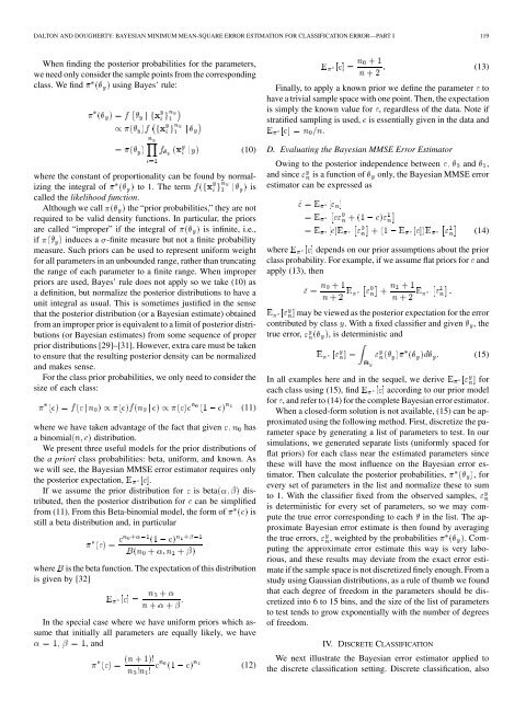
DALTON AND DOUGHERTY: BAYESIAN MINIMUM MEAN-SQUARE ERROR ESTIMATION FOR CLASSIFICATION ERROR—PART I 119When finding the posterior probabilities for the parameters,we need only consider the sample points from the correspondingclass. We find using Bayes’ rule:(10)where the constant of proportionality can be found by normalizingthe integral of to 1. The term iscalled the likelihood function.Although we call the “prior probabilities,” they are notrequired to be valid density functions. In particular, the priorsare called “improper” if the integral of is infinite, i.e.,if induces a -finite measure but not a finite probabilitymeasure. Such priors can be used to represent uniform weightfor all parameters in an unbounded range, rather than truncatingthe range of each parameter to a finite range. When improperpriors are used, Bayes’ rule does not apply so we take (10) asa definition, but normalize the posterior distributions to have aunit integral as usual. This is sometimes justified in the sensethat the posterior distribution (or a Bayesian estimate) obtainedfrom an improper prior is equivalent to a limit of posterior distributions(or Bayesian estimates) from some sequence of properprior distributions [29]–[31]. However, extra care must be takento ensure that the resulting posterior density can be normalizedand makes sense.For the class prior probabilities, we only need to consider thesize of each class:(11)where we have taken advantage of the fact that given hasa binomial distribution.We present three useful models for the prior distributions ofthe a priori class probabilities: beta, uniform, and known. Aswe will see, the Bayesian MMSE error estimator requires onlythe posterior expectation, .If we assume the prior distribution for is beta distributed,then the posterior distribution for can be simplifiedfrom (11). From this Beta-binomial model, the form of isstill a beta distribution and, in particularwhere is the beta function. The expectation of this distributionis given by [32]In the special case where we have uniform priors which assumethat initially all parameters are equally likely, we have, and(12)(13)Finally, to apply a known prior we define the parameter tohave a trivial sample space with one point. Then, the expectationis simply the known value for , regardless of the data. Note ifstratified sampling is used, is essentially given in the data and.D. Evaluating the Bayesian MMSE Error EstimatorOwing to the posterior independence between and ,and since is a function of only, the Bayesian MMSE errorestimator can be expressed as(14)where depends on our prior assumptions about the priorclass probability. For example, if we assume flat priors for andapply (13), thenmay be viewed as the posterior expectation for the errorcontributed by class . With a fixed classifier and given , thetrue error, , is deterministic and(15)In all examples here and in the sequel, we derive foreach class using (15), find according to our prior modelfor , and refer to (14) for the complete Bayesian error estimator.When a closed-form solution is not available, (15) can be approximatedusing the following method. First, discretize the parameterspace by generating a list of parameters to test. In oursimulations, we generated separate lists (uniformly spaced forflat priors) for each class near the estimated parameters sincethese will have the most influence on the Bayesian error estimator.Then calculate the posterior probabilities, , forevery set of parameters in the list and normalize these to sumto 1. With the classifier fixed from the observed samples,is deterministic for every set of parameters, so we may computethe true error corresponding to each in the list. The approximateBayesian error estimate is then found by averagingthe true errors, , weighted by the probabilities . Computingthe approximate error estimate this way is very laborious,and these results may deviate from the exact error estimateif the sample space is not discretized finely enough. From astudy using Gaussian distributions, as a rule of thumb we foundthat each degree of freedom in the parameters should be discretizedinto 6 to 15 bins, and the size of the list of parametersto test tends to grow exponentially with the number of degreesof freedom.IV. DISCRETE CLASSIFICATIONWe next illustrate the Bayesian error estimator applied tothe discrete classification setting. Discrete classification, also
Page 1 and 2: IEEE TRANSACTIONS ON SIGNAL PROCESS
Page 3: DALTON AND DOUGHERTY: BAYESIAN MINI
Page 7 and 8: DALTON AND DOUGHERTY: BAYESIAN MINI
Page 15: DALTON AND DOUGHERTY: BAYESIAN MINI

Bayesian Minimum Mean-Square Error Estimation for ... - IEEE Xplore

You also want an ePaper? Increase the reach of your titles

Delete template?

Save as template?