Distributing labels on infinite trees

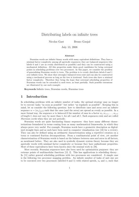
<strong>Distributing</strong> <strong>labels</strong> on infinite treesNicolas GastBruno GaujalJuly 13, 2008AbstractSturmian words are infinite binary words with many equivalent definitions: They have aminimal factor complexity among all aperiodic sequences; they are balanced sequences (the<strong>labels</strong> 0 and 1 are as evenly distributed as possible) and they can be constructed using amechanical definition. All this properties make them good candidates for being extremalpoints in scheduling problems over two processors. In this paper, we consider the problemof generalizing Sturmian words to trees. The problem is to evenly distribute <strong>labels</strong> 0 and 1over infinite trees. We show that (strongly) balanced trees exist and can also be constructedusing a mechanical process as long as the tree is irrational. Such trees also have a minimalfactor complexity. Therefore they bring the hope that extremal scheduling properties ofSturmian words can be extended to such trees, as least partially. Such possible extensionsare illustrated by one such example.Keywords Infinite trees, Sturmian words, Sturmian trees1 IntroductionIn scheduling problems with an infinite number of tasks, the optimal strategy may no longerbe to execute tasks “as soon as possible” but rather “as regularly as possible”. Keeping this inmind, let us consider the following question: how to distribute ones and zeros over an infinitesequence w = (w n ) n∈N such that the ones (and the zeros) are spread as evenly as possible. In amore formal way, the sequence w is balanced if the number of ones in a factor w i , w i+1 , . . . , w i+lof length l, does not vary by more than 1, for all i and all l. Such sequences exist and are calledSturmian words when they are not periodic.Sturmian words are quite fascinating binary sequences: they have many different characterizationsformulated in terms coming from as many mathematical frameworks, in which theyalways prove very useful. For example, Sturmian words have a geometric description as digitalizedstraight lines and as such have been used in computer visualization (see [13] for a review).They can also be defined using an arithmetic characterization using a repetitive rotation on atorus or continued fraction decompositions. From a combinatorial point of view, yet anothercharacterization of Sturmian words is based on the balance between ones and zeros in all factors,as mentioned before. They are also used in symbolic dynamic system theory because they areaperiodic words with minimal factor complexity or because they have palindromic properties.Most of these equivalences have been known since the seminal work in [16].More recently, Sturmian sequences have also been used for optimization purposes: they areextreme points of multimodular functions [12, 2]. This has applications is scheduling theory .In [11] rather general scheduling problems with two processors are considered. A simple caseis the following two processor mapping problem. An infinite number of tasks of unit size areto be executed over two processors (labeled 0 and 1) with related speeds, v 0 and v 1 such that1

1/v 0 + 1/v 1 > 1. The tasks are released every time unit. It is shown that an optimal schedule(minimizing the average flow time) allocates task i to processor w i according to a sequencew 1 , w 2 , w 2 , . . . that is Sturmian.Another example solved in [10] is the following processor allocation problem: A single processor(with unit speed) is used to execute two types of tasks. Tasks of type 1 (resp. 2) arereleased every time unit and are all of size S 0 (resp. S 1 ). The allocation of the processor to thetasks can be seen as a binary sequence w 1 , w 2 , . . . saying which task is to be served next. Herealso there exists an optimal Sturmian. sequence (minimizing the average flow time of all tasks).Actually more general scheduling problems are solved by Sturmian sequences. For instanceof the tasks are released according to a stationary process and the task sizes are also stochastic,independent of the release process, then both problems mentioned above are also solved bySturmian sequences.A natural extension is to consider the case where more than two processors can be usedto execute the tasks. This leads to the construction of generalized Sturmian words in severaldirection.The first one is to study words using more than two letters. Billiard sequences in hypercubesextent the torus definition of Sturmian sequences while episturmian sequences [3] extend thepalindromic characterization of Sturmian words. Unfortunately, both extensions differ substantiallyand none of them provides an optimal schedule for the k processor mapping problem.Another extension is to two dimensions. A complete characterization of two-dimensionalnon-periodic sequences with minimal complexity is given in [6]. Here again the alternativecharacterizations are lost.Yet another generalization is to trees [4], where Sturmian trees are defined as infinite binaryautomata such that the number of factors (sub-trees) of size n is n+1. The other characterizationsof Sturmian words are lost once more.Finally, another extension of Sturmian concerns discrete planes. Here, several characterizationsof Sturmian lines can be extended to discrete planes. Interesting relations betweenmultidimensional continued fraction decomposition of the normal direction of the plane and thepatterns of its discretization mimic what happens for Sturmian sequences, [8].The aim of this paper is to do the same for trees. We introduced in [9] a new type of infinitetrees: unordered trees, for which the left and right children of each node are not distinguishableand gave a brief presentation of its main properties. Here, We make an exhaustive study ofsuch trees. We show that the balance property (distributing evenly the <strong>labels</strong> equal to one orzero over the vertex of the tree) coincides with a characterization of trees using integer parts ofaffine functions (called mechanicity). Furthermore these balanced trees have a minimal factorcomplexity. Therefore, they can be seen as a natural extension of Sturmian sequence in morethan one aspect. This brings some hope to use them as extreme points for adapted optimizationproblems.Our purpose in the paper is two-fold. The first part of the paper is dedicated to the study ofgeneral unordered infinite trees with binary <strong>labels</strong>. We provide definitions of the main conceptsas well as the basic properties of unordered trees with a special focus on the notion of density(the average number of ones) and rationality The second part of the paper investigates balancedunordered trees and their properties. In particular we show that strongly balanced trees (definedlater) are mechanical (so that they have a density and all <strong>labels</strong> can be constructed in almostconstant time). Furthermore their factor complexity is minimal among all non-periodic trees.We also investigate rational balanced trees by showing that their density is easy to computeand by providing an algorithm with polynomial complexity to test whether a rational tree isstrongly balanced. Finally, we show that balanced trees are extremal points of some convexfunctions, bringing some hope that they can be used to solve optimization problems.2

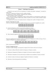
2 Infinite TreesFor ordered infinite trees , we follow the presentation given in [4]. Ordered infinite trees areautomata with an infinite number of states. An automata is a tree-automaton if it has oneinitial state and each state has a uniform in-degree equal to one (except for the initial state,whose in-degree is 0) and a uniform out-degree d with <strong>labels</strong> a 1 , · · · , a d on the arcs. Every nodev is labeled by l(v) = 1 (resp. 0) if it is final (resp. non-final).The language accepted by the tree-automaton T is a subset of A ∗ (where the alphabetA = {a 1 , . . . a d }) and is denoted by L(T ). Thus, a word w in the free monoid A ∗ correspondsto a node in T , and a word w in L(T ) corresponds to a node in T with label 1. Conversely, aunique tree-automaton can be associated to any subset L of A ∗ , by labeling by one the nodescorresponding to the words in L.Classically for automata, a family of equivalence relations can be defined over the nodes oftree T : v ∼ 0 u if l(v) = l(u), v ∼ n+1 u if v ∼ n u and for all i, the ith child of u, ua i and the ithchild of v, va i satisfy ua i ∼ n va i . By definition of ∼ n , u ∼ n v if and only if the subtree rootedin u of height n is the same as the subtree rooted in v of height n.L(T ) is recognized by its minimal deterministic automaton (possibly infinite), say A(T ).Actually, A(T ) can be obtained from the tree T by merging all the states in the tree in the sameequivalence classes of ∼ n for all n.An example is given in Figure 1 where the infinite tree-automaton and the minimal automatonrecognizing all the prefixes of the Fibonacci word (over the alphabet {a, b}) is given together withthe corresponding minimal automaton (which has an infinite number of states).abababa b a a b a b0 1 2 3 4 5 6...b a b b a b a∞a,bFigure 1: The tree-automaton recognizing the Fibonacci word and the corresponding minimalautomatonThe number of subtrees of size k in T is called the complexity P (k), of T . P (k) is the numberof equivalence classes of ∼ k . If P (k) ≤ k for at least one k, then it can be shown ([4]) that thecomplexity is bounded by k. This implies that the minimal automaton A(T ) has k states. Thetree is therefore called rational, since it recognizes a rational language.If a tree-automaton T is such that P (k) = k + 1 for all k, then it has a minimal complexityamong all non-rational trees. Such trees have been shown to exist and are called Sturmian in[4] by analogy with the factor complexity definition of Sturmian words. In [4] several classesof Sturmian tree-automata are presented. However such trees are not balanced and cannot bedefined using a mechanical construction, as with Sturmian words.3

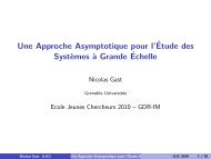
In the following we rather consider a different type of trees, namely infinite directed graphswith <strong>labels</strong> 0 or 1 on nodes and with uniform in-degree 1 and out-degree d ≥ 2. Here, the childrenof a node are not ordered. Thus, the main difference with the previous definition is that arcs arenot labeled. Therefore such trees cannot be bijectively associated with languages. However, it ispossible to construct a minimal multi-graph (i..e. with multiples arcs) G(T ) associated with thetree T , mimicking the construction of the minimal automaton for ordered trees. Let us considera family of equivalence relations over the nodes of T :v ≡ 0 u if u and v have the same label: l(u) = l(v) andv ≡ n+1 u if v ≡ n u and the children of v are equivalent (for ≡ n ) to the children of u.Therefore, v ≡ n u if and only if the subtree with root v of height n is isomorphic to the subtreewith root u with height n. By merging the nodes of T when they belong to the same equivalenceclasses, for all n, one gets the minimal multi-graph G(T ) of the factors of T : all nodes mergedin the same vertex of G(T ) have the same subtrees of every height.In G(T ), the node corresponding to the root of T is distinguished. (graphically, this is doneby adding an arrow pointing to the node).There exists a way to associate an ordered tree-automaton T to a tree T by choosing an orderon the children of each node. This can be done by seeing G(T ) as an automaton by labeling arcsin G(T ) with letters a 1 , . . . a d in an arbitrary fashion. Conversely, a tree-automaton T can beconverted into a graph T by removing the <strong>labels</strong> on the arcs. This graph is called the unorderedversion of T .An example of an unordered tree is given in Figure 2. The label of the black (white) node is 1(0). The arcs are implicitly directed from top to bottom. Actually, most figures in this paper willrepresent binary trees (with out-degree d = 2), although all the discussion is carried throughoutfor arbitrary degrees. The nodes of the associated multi-graph G(T ) are numbered arbitrarilyand nodes with label 1 are displayed with a bold circle. The node corresponding to the rootof the tree is pointed by an arrow. This tree can be seen as the tree-automata recognizing theFibonacci word where the <strong>labels</strong> on the arcs have been removed (there is no longer a left andright child at each node). Note that while the minimal automaton is infinite (see Figure 1), theminimal graph G(T ) is finite, with two nodes, one correspond to the tree where all <strong>labels</strong> are 0and one with all <strong>labels</strong> equal to 0 expect on one branch (see Figure 2).0∞Figure 2: A tree and the associated minimal multi-graph.4

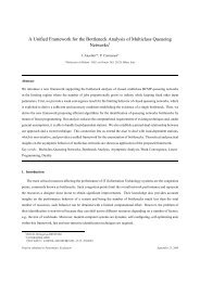
2.1 Irreducibility and periodicityBy analogy with Markov chains, a tree T is irreducible if G(T ) is strongly connected. Also, anirreducible tree T is periodic with period p if the greatest common divisor of the lengths of allcycles in G(T ) is p. A tree with period 1 is also called aperiodic.2.2 Factors, complexity and Sturmian treesA factor of size n (and width 1) is a subgraph of T which is a complete subtree of height n. Thenumber of nodes in a factor of size n is denoted by S(n) def= dn −1d−1 .A factor of size n and width k (with root v), is a sub-graph of T which is the subtree of heightk + n rooted in v minus the subtree of height k, rooted in v. The number of nodes of a factor ofsize n and width k is S(n, k) def= dn+k −d kd−1.Similarly to what as been done for words, the factor complexity P T (n) of a tree T is thenumber of distinct factors of size n and width 1.The complexity of a tree P T (n) can be bounded by the total number of ways to label treesof height n and degree d, say A n .It should be clear that A 1 = 2 (a node can be labeled 0 or 1) and that A n+1 = 2M(A n , d)where M(x, y) is the number of multisets with y elements taken from a set with x elements.Therefore using binomial coefficients,( )An + d − 1A n+1 = 2.A n − 1This is a polynomial recurrence equation of degree d. A change of variable, u n = log A n +1d−1 log 2 d! yields a new recurrence equation u n+1 = du n + ε n where ɛ n = o(1). This implies thatA n = φ dn +o(d n) for some φ with 1 < φ < 2.As for lower bounds on the complexity of a tree, it will be shown in Section 3 that trees suchthat P T (n) ≤ n for at least one n are rational, i.e. have a bounded number of factors of any size(this means that the minimal multi-graph is finite).Therefore, trees T such that G(T ) is infinite and with a minimal complexity should satisfyP T (n) = n+1. These trees will be called Sturmian trees by analogy with words. It is not difficultto exhibit such trees. For example, starting with a Sturmian word w a binary tree such that allnodes on level i have label w i is Sturmian.Another more interesting example is the Dyck tree. The Dyck tree is represented on Figure 3.This tree is the unordered version of the tree-automata recognizing the Dyck language (languagegenerated by the context-free grammar S → aSbS|ɛ) and it is not hard to see that this tree isSturmian. For that, consider the graph G(T ) associated with the Dyck tree T , also displayed inFigure 3.There are two factors of size 1 in T : those with a root labeled 1 (all associated with node0 in G(T )) and those with a root labeled 0 (associated with nodes ∞, 1, 2, · · · in G(T )). Thiscorresponds to the equivalence classes for ≡ 1 .As for factors of size n, all those with a root in node ∞ and n, n+1, n+2 have all their <strong>labels</strong>equal to 0: no path of length n in G(T ) reaches the only node with label 1, namely node 0.As for the factors starting in node i of G(T ) with 0 ≤ i < n, then the first node with label 1is at level i + 1. This means that all these factors are distinct. In other words, the equivalenceclasses for ≡ n are {∞, n, n + 1, . . .}, {0}, {1}, . . . , {n − 1}. The number of distinct factors of sizen is therefore n + 1.5

∞ 0 1 2 3 4 5 ...Figure 3: The Dyck tree and its minimal graph.2.3 DensityThe density of a tree T is meant to capture the average number of 1 in the tree.For a node v and a height n ≥ 0, we define the density of the factors of size n with root v bythe average number of nodes with label 1 in this sub-tree. Let us call d v (n) the density of thefactor of size nwith root v and let r be the root of the tree T . In the following we will be usingfour notions of density.• The rooted density of the tree is the limit of the density of the sub-trees of the root r (if itexists):limn→∞ d r(n)• The rooted average density of the tree the Cesaro limit of these densities:1limn→∞ nn∑d r (n)• The density of the tree is α if it has an identical rooted density for all node v:i=1∀v : α = limn→∞ d v(n)• The average density of the tree is α if it has an identical rooted average density for all nodev:1n∑∀v : α = lim d v (n)n→∞ nFrom the definition, we have the following direct implications: If a tree admits a density, thenit admits an average density. In turn, a tree with a average density also has a rooted averagedensity. Also, a tree with a density has a rooted density.Although the rooted definitions seem more natural and simple , the definition of generaldensities have the advantage that they do depend on the choice of the root. See Figure 4 forsome examples. These examples will be further developed in the following section on rationaltrees.i=16

Figure 4: The first tree has a density of 1/2, the second one an average density equal to 1/2 butno density. The last one has a rooted density 1/2 but no average density.3 Rational treesA tree T is rational if the associated minimal multi-graph G(T ) is finite.An example of a rational tree T is displayed in Figure 5 together with its graph G(T ). Notethat this tree is not irreducible. One final strongly component of period 2 (it corresponds to thealternating subtrees starting with ones and zeros displayed on the left) while the other one isaperiodic (it corresponds to the subtree with all its <strong>labels</strong> equal to one, displayed on the right).1234Figure 5: A rational tree made of two distinct subtrees and its associated multi-graphIt is possible to characterize rational trees using their complexity.Theorem 3.1. The following proposition are equivalent1. the tree T is rational;2. there exists n such that P(n) ≤ n;3. there exists n such that P(n) = P(n + 1);4. There exists B such that for all n, P(n) ≤ B.Proof. The proof of this results is similar to the proof for words.1 implies 2: If G(T ) is finite, then the number of factors of size n in T is smaller than the sizeof G(T ), therefore, there exists n such that P(n) ≤ n.2 implies 3: Since P(1) = 2 and P(n) ≤ n and since P is non-decreasing with n, there exists1 < k < n such that P(k) = P(k + 1).3 implies 4: If P(n) = P(n + 1) = p then let us call by A n 1 , . . . A n p all the distinct factors of sizen in T . Since P (n + 1) = p, each A n i is prolonged in a unique way into a tree of size n + 1,7

called A n+1i . Now, each sub-tree A n+1i is composed of a root and d factors of size n, in the set{A n 1 , . . . A n p }. In turn, they are all prolonged into trees of size n in a unique way. Therefore,P(n + 2) = p. By a direct induction, P(k) = p for all k ≥ n.4 implies 1: If the number of factors of size n is smaller than B for all n, then this means thatthe number of equivalence classes for ≡ n is smaller than n for all n, this means that G(T ) hasless than B nodes.3.1 Density of rational treesLet T be a rational tree and let G(T ) be its minimal multi-graph. The nodes of G(T ) arenumbered v 1 · · · , v K , with v 1 corresponding to the root of T .G(T ) can be seen as the transition kernel of a Markov chain by considering each arc of G(T )as a transition with probability 1/d.If G(T ) is irreducible then the Markov chain admits a unique stationary measure π on itsnodes. The density of T and the stationary measure π are related by the following theorem.Theorem 3.2. Let T be an irreducible rational tree with a minimal multigraph G(T ) with Knodes. Let l = (l 1 , . . . l K ) be the <strong>labels</strong> of the nodes of G(T ) and let π = (π 1 , . . . , π K ) be thestationary measure over the nodes of G(T ).If T is aperiodic, then T admits a density α = πl t .If T is periodic with period p then T admits an average density α = πl t .Proof. Let V n be a Markov chain corresponding to G(T ). Since G(T ) is irreducible, V n admits aunique stationary measure , say π = (π 1 , . . . , π K ). Let us call P the kernel of this Markov chain:P i,j = a/d if there are a arcs in G(T ) from v i to v j .Now, let us consider all the paths of length n in T , starting from an arbitrary node v i . Byconstruction of G(T ), the number of paths that end up in the nodes v 1 , · · · , v K respectively, ofG(T ), is given by the vector e i d n P n , where e i is the vector with all its coordinates equal to 0except the ith coordinate, equal to 1.∑ n−1Now, the number of ones in the tree of height n starting in v i is h n (v i ) = e i k=0 dk P k l t .Let us first consider the case where P is aperiodic. We denote by Π the matrix with all itslines equal to the stationary measure, π and by D k the matrix P k − Π. When P is aperiodic,then lim k→∞ ||D k || 1 = 0. Therefore, for all k > n, ||D k || 1 < ɛ n → 0.Then the density of ones d 2n (v i ) =size 2n into a factor of size n at the root and d. factors of size n. One getsd−1d 2n −1 h 2n(v i ) can be estimated by splitting the factors ofd 2n (v i ) ==d − 1d 2n − 1 e id − 1d 2n − 1 e i(n∑k=1d k P k l t + d − 1d 2n − 1 e in∑d k P k +k=12n−1∑k=n+1d k D k +2n−1∑k=n+12n∑k=n+1d k P k l t ,d k Π)l t .∑ nwhen n goes to infinity, the first term goes to 0 because e i k=1 dk P k l t ≤ d n+1 . As for thesecond termd−1d 2n −1 e ∑ 2n−1i k=n+1 dk D k l t ≤ 1d 2n −1 d2n ɛ n . This goes to 0 when n goes to infinity.d−1As for the last term,d 2n −1 e ∑ 2n−1i k=n+1 dk Πl t = 1d 2n −1 (d2n −d n+2 )(e i Π)l t this goes to πl t whenn goes to infinity.The same holds by computing the density of trees of size 2n + 1 by splitting them into thefirst n + 1 levels and the last n levels.This shows that the rooted density of all the trees in T is the same, equal to πl t .8

Let us now consider the case when the tree is periodic with period p. In that case, the kernelof p steps of the Markov chain can be put under the form⎡P 1 0 · · · 0⎤0 0 . . . P m .P p =0 P .. 2 0⎢⎣.. .. . ⎥ .. . ⎦ .The sub-matrices P 1 , . . . , P m are the kernels of aperiodic chains defined on a partition S 1 . . . S mof the nodes of G(T ). Let us denote by α 1 , . . . α m the densities of the factors of size np, startingin S 1 . . . S m , respectively (they exist because this has just been proved for aperiodic trees).Starting from a node v the average density of a tree of size n = pq n + r n , r n < p is1nn∑1 ∑q nd k (v) = (pq n + r nk=0a=0 b=0p∑1d ap+b+r (v) +pq n + r nr n∑k=0d k (v)).The first term goes to (α 1 + . . . + α m )/m while the second term goes to zero, when n goes toinfinity, independently of the root. Finally, (α 1 + . . . + α m )/m = (π ′ 1l t 1 + · · · + π ′ ml t m)/m = πl twhere π ′ 1, · · · , π ′ m are the stationary probability for the kernels P 1 , . . . , P m and l 1 , . . . l m are thevectors of the <strong>labels</strong> in S 1 . . . S m .12 3Figure 6: An irreducible aperiodic rational tree and its minimal graph. The stationary probabilitiesover the associated Markov chain are π = (2/9, 3/9, 4/9). The density of the tree isα = 4/9.An example illustrating the computation of the density of an aperiodic irreducible rationaltree is given in Figure 6. The stationary measure of the Markov chain is π = (2/9, 3/9, 4/9).Therefore, the density is α = 2/9l 1 + 3/9l 2 + 4/9l 3 = 4/9.As for the reducible case, it should be easy to see that a rational tree may have different(average) densities for some of its subtrees (this is the case for the leftmost tree in Figure 4).Therefore, a reducible tree does not have a density nor an average density in general.Let us call S 1 , · · · , S m the final strongly connected components of G(T ). Let α 1 , . . . , α m bethe average densities of the components S 1 . . . , S m respectively. Finally, let R = (R 1 · · · R m ) bethe probability of reaching the components S 1 · · · S m starting from the root v 1 , in the Markovchain associated with G(T ). Then, the following is true.Theorem 3.3. A rational tree always has a rooted average density α = (α 1 , . . . α m )R t .9

Proof. If P is reducible, P can be decomposed into⎡⎤⎡Q K 1 · · · K m0 P 1 · · · 0P = ⎢⎣.. . . . ..⎥. ⎦ and P n = ⎢⎣0 0 . . . P mQ n K 1 ′ · · · K m′0 P1 n · · · 0.. . . . .. .0 0 . . . Pmn⎤⎥⎦Considering all the paths in G(T ) of length n, starting in the root, the number of pathsending in component S l is N l (n) = d n ∑ i∈S lP1i n. Let us decompose all the paths ending in S linto two sub-paths: one (of length k) before entering S l and one (of length n − k) inside S l , weget from the decomposition of P n , N l (n) = d n ∑ nk=0 (1, 0, . . . , 0)Qk K l u l , where u l is a vectorwhose coordinates are 1 in S l and 0 everywhere else.The number of 1 in the rooted subtree of T of size 2n is the number of ones in all the pathsof length n plus the number of ones in the subtrees of size 1. When n is large, the number ofones in the paths can be neglected with respect to the number of ones in the end trees.Finally, the number of one in a tree of size 2n is the number of ones in each possible end-treeof size n times the number of such trees, namely N l (n). When n goes to infinity, the density ofones goes to ∑ l=1..m α l(1, 0, . . . , 0)(I − Q) −1 K l u l = (α 1 · · · α m )R t , with R l = (1, 0, . . . , 0)(I −Q) −1 K l u l .An example illustrating the computation of the rooted average density of a tree is given inFigure 5. The graph G(T ) has two final components, one aperiodic component with density 1 andanother one with period 2 with average density 1/2. Starting from the root, both componentsare reached with probability 1/2. Therefore, such a tree has an average rooted density α =1/2(1/2) + 1/2(1) = 2/3.Also, it is not difficult to show that if all final component have a density (rather than anaverage density), then the tree has a rooted density, given by the same formula as in Theorem3.3.Finally, it is fairly straightforward to prove that since the K · K kernel P of the Markov chainassociated with G(T ) has all its elements of the form a/d, then the stationary probabilities π aswell as the average rooted density α of a rational tree are rational numbers of the form c/b with0 ≤ c ≤ b ≤ d K+1 . This fact will be used in the algorithmic section 5 to make sure that thecomplexity of the algorithms does not depend on the size of the numbers.4 Balanced and Mechanical TreesIn this section, we will introduce our most important definitions: strongly balanced and mechanicaltrees and explore the relations between them. In particular we will prove that in the caseof irrational trees they represent the same set of trees, giving us a constructive representation ofthis class of trees. These results are very similar to the ones on words, which are summarizedbelow.4.1 Sturmian, Balanced and Mechanical WordsOne definition of a Sturmian word uses the complexity of a word. The complexity of an infiniteword w is a function P w : N → N where P w (n) is the number of distinct factors of length n of theword w. A word is periodic if there exists n such that P w (n) ≤ n. Sturmian words are aperiodicwords with minimal complexity, i.e such that for any n:P w (n) = n + 1. (1)10

If x is a factor of w, its height h(x) is the number of letters equal to 1 in x. A balanced word isa word where the letters 1 are distributed as evenly as possible:∀x, y factors of w, |x| = |y| ⇒ |h(x) − h(y)| ≤ 1. (2)A mechanical word is constructed using integer parts of affine functions. Let α ∈ [0; 1] andφ ∈ [0; 1). The lower (resp. upper) mechanical word of slope α and phase φ, w = w 1 w 2 . . . (resp.w ′ = w 1w ′ 2 ′ . . . ) is defined by:∀i ≥ 1w i = ⌊(i + 1)α + φ⌋ − ⌊nα + φ⌋,w ′ i = ⌈(i + 1)α + φ⌉ − ⌈iα + φ⌉. (3)These three definitions represent almost the same set of words. In the case of aperiodic words,they are equivalent: a word is Sturmian if and only if it is balanced and aperiodic if and only ifit is mechanical of irrational slope. For periodic words, there are similar relations:• A rational mechanical word is balanced.• A periodic balanced word is ultimately mechanical.A word is an ultimately mechanical word if it can written as xw where x is a finite word and w isa mechanical word. An example of a balanced word which is not mechanical (and just ultimatelymechanical) is the infinite word with all letter 0 and just one letter 1. For a more completedescription of Sturmian words, we refer to [14].4.2 Balanced and strongly balanced treesUsing the two definitions of factors of a tree, we define two notions of balance for trees: the firstone and probably the most natural one, is what we call balanced trees and the other one is calledstrongly balanced trees.Definition 4.1 (Balanced and strongly balanced tree). A tree is balanced if for all n ≥ 0, thenumber of nodes label by 1 in two factors of size n differ by at most 1.A tree is strongly balanced if for all n, k > 0, the number of 1 in two factors of size n andwidth k differ by at most 1.As the name suggests, the strong balance property implies balance (by taking k = 1). Infact this notion is strictly stronger, see section 7 for an example of balanced tree that are notstrongly balanced.Although the balance property is weaker and seems more natural for a generalization fromwords, our results will be mainly focused on strongly balanced trees that have almost the sameproperties as their counterparts on words.4.2.1 Density of a balanced treeFor all node v and all size n, we denote by h v (n) the number of 1 in the factor of root v of size nand d v (n) the density of this subtree is the number of ones divided by the cardinal S(n) of thefactor: d v (n) def= 1S(n) h v(n).Proposition 4.1.1 (Density of balanced tree). A balanced tree has a density α.Moreover for all node v and for all size n:|h v (n) − ⌊S(n)α⌋| ≤ 1 (4)11

Proof. Let m n be the minimal number of 1 in all factors of size n. As the tree is balanced, forall nodes v and n ≥ 1:m n ≤ h v (n) ≤ m n + 1 (5)Now let us consider a factor of size n + k and root v. It can be decomposed in a factor of sizek of root v and d k factors of size n at the leaves of the previous factor. The number of ones inthese factors can be bounded by m n and m k , therefore we have:m k + d k m n ≤ m n+k ≤ m k + 1 + d k (m n + 1) (6)The density of a factor of size n is mnS(n) ≤ d v(n) = hv(n)S(n)bound d v (n + k) − d v (n):≤ mn+1S(n). Using these facts, we canm n+kS(n + k) − m n + 1≤ d v (n + k) − d v (n) ≤ m n+k + 1S(n)S(n + k) − m nS(n)Using (6), the left inequality can be lower bounded by(d − 1) ( d k m n + m kd n+k − 1 − m n + 1)d n − 1= (d − 1) ( m n + m k /d kd n − 1/d k − m n + 1)d n − 1)≥ (d − 1) ( m nd n − 1 − m n + 1d n − 1≥ − 1S(n)The same method can be used to prove that d v (n + k) − d v (n) ≤ 1S(n), which shows thatfor n big enough, |d v (n + k) − d v (n)| is smaller than ɛ, regardless of k. Thus d v (n) is a Cauchym nS(n)sequence and has a limit α = lim n→∞ . This limit does not depend on v and the tree has adensity.Lets now prove that d v (n) − ⌊S(n)α⌋| ≤ 1: dividing the inequality (6) by S(n, k) and takingthe limit when k tends to ∞ leads to:(d − 1)m n + αd n≤ α ≤ (d − 1)m n + 1 + αd n .This shows that: S(n)α − 1 ≤ m n ≤ S(n)α, which implies Equation (4).Similar ideas can be used to show that Equation (4) can be improved in the case of stronglybalanced tree: for all width and size k, n ≥ 1, the number of ones h(n, k) in a factor of size nand width k satisfies:∣ h(n, k) − ⌊S(n, k)α⌋∣ ∣ ≤ 1 (7)4.3 Mechanical treesBuilding balanced tree is not that easy. According to formula (4), each factors of size n musthave ⌊αS(n)⌋ or ⌊αS(n)⌋ + 1 nodes one. This leads us to the following construction, inspired bythe construction of mechanical words.12

Definition 4.2 (Mechanical tree). A tree is mechanical of density α ∈ [0; 1] if for all node v,there exists a phase φ v which satisfies one of the two following properties:⌋∀n : h v (n) =⌊S(n)α + φ v , (8)⌉or ∀n : h v (n) =⌈S(n)α − φ v . (9)In the first case, we say that φ v is an inferior phase of v. In the second case, we say that φ vis a superior phase of v.This definition suggests that the phases of all nodes could be arbitrary. In fact, we will seethat there exists a unique mechanical tree with a given phase at the root. The second questionraised by this definition is the existence and uniqueness of the phase: we call φ v “a” phase of anode φ v and not “the” phase of φ v since there may exist several phases leading to the same tree.We begin by a characterization of mechanical trees, given in the following formula:Proposition 4.2.1 (Characterization of mechanical trees). For each α ∈ [0; 1] and φ ∈ [0; 1),there exists a unique mechanical tree of density α such that φ is an inferior (resp. superior)phase of the root.Moreover, if φ is an inferior (resp. superior) phase of a node then φ 0 ≤ · · · ≤ φ d−1 areinferior (resp. superior) phases of its d children, withφ i =α + φ + i − ⌊α + φ⌋d(resp. φ v =)φ + ⌈α − φ⌉ − α + i. (10)dThe proof will be done in two steps. First we will see that if we define the phases as in (10)we have a mechanical tree, then we will see that this is the only way to do so.Proof. Existence. Let α ∈ [0; 1] and φ ∈ [0; 1). We want to build a mechanical tree whichroot has an inferior phase φ ( the case of a superior phase if similar and is not detailed here).Let A be an infinite tree. To each node v, we associate a number φ v defined by:• φ root = φ.• If the phase of a node v is φ v , its d children satisfy Equation (10).Then we build a labeled tree by associating to each node v the label ⌊α + φ v ⌋. Let us prove byinduction on n that the following relation holds.⌋For all v : h v (n) =⌊S(n)α + φ v . (11)By definition of the <strong>labels</strong>, (11) holds when n = 1. Let n ≥ 0 and let us assume that (11) holdsfor n. Let v be a node with phase φ v and let φ 0 . . . φ d−1 be the phases of its children. We assumethat α + φ v < 1 (which means that the label of the node is 0) a similar calculation can be donein the other case, α + φ v > 1.13

Using the well-known formula ∑ d−1i=0 ⌊x + i d ⌋ = ⌊dx⌋, we can compute h v(n + 1):h v (n + 1) ==∑d−1⌊S(n)α + φ i ⌋i=0∑d−1⌊ dn − 1d − 1 α + α + φ + i ⌋di=0= ⌊d( dn − 1d − 1 α + α + φ )⌋d= ⌊S(n + 1)α + φ⌋.Therefore, (11) holds for all n which means that the tree is mechanical.Uniqueness. Now, let A be a mechanical tree of density α. Let v be a node and φ 0 , . . . , φ d−1be the phases of its children. Let i and j be two children and let h i (n) be the number of onesin the ith child subtree (of phase φ i ). We want to prove that either for all n: h i (n) ≤ h j (n) orfor all n: h i (n) ≥ h j (n). If the two nodes are both inferior (resp. superior), this is clearly true:h i (n) ≤ h j (n) if and only if φ i ≤ φ j (resp. φ i ≥ φ j ). If i is inferior and j is superior, it is notdifficult to show that φ i < 1 − φ j implies h i (n) ≤ h j (n) and φ i ≥ 1 − φ j implies h i (n) ≥ h j (n).Therefore we can assume (otherwise we exchange the order of the children) that for all n:h 0 (n) ≤ h 1 (n) ≤ · · · ≤ h d−1 (n).Moreover as h d−1 (n) − h 0 (n) ≤ 1, there exists k such that h 0 (n) = h 1 (n) = · · · = h k (n) φ, ψ is nota phase of the node. Conversely, if the exists δ > 0 such that frac(S(n)α + φ) > δ (resp. < 1 − δ)for all n, then let φ ′ = φ − ε (resp. φ ′ = φ + ε), with ε < δ. Then ⌊S(n)α + φ⌋ = ⌊S(n)α + φ ′ ⌋for all n.Finally, a phase φ is unique if and only if 0 and 1 are accumulation points of the sequence{frac(S(n)α + φ)} n∈N.Let us call x def= 1defd−1α and y = φ − x and let us consider the sequencefrac(S(n)α + φ) = frac(xd n − y).14

Let x 1 , . . . , x k , . . . (resp. y 1 , y 2 , . . . ) be the sequence of the digits of x (resp. y) in base d (alsocalled the d-decomposition). We have:xd n − y =n∑∞∑x k d n−k + (x k+n − y k )d −kk=1} {{ }∈Nfrac(xd n − y) is arbitrarily close to 0 implies that for arbitrarily big k, there exists n such thatork=1x n , . . . , x n+k−2 = y 1 , . . . , y k , x n+k−1 > y n , (12)frac(xd n − y) = 0. (13)Also, xd n − y is arbitrarily close to 1 implies that for arbitrarily big k, there exists n such thatx n , . . . , x n+k−2 = y 1 , . . . , y n−1 , x n+k−1 < y n , (14)or the d-development of y is finite (with only zeros after some point l : y = y 1 , . . . , y l , 1, 0, 0 . . .)and that for arbitrarily big k, there exists n such thatx n , . . . , x n+k−2 = y 1 , . . . , y l , 0, 1, . . . , 1. (15)Using this characterization, three cases can be distinguished.α• Ifd−1is a number such that all finite sequences over 0, . . . , d−1 appear in its d-decomposition,then every phase is unique. In particular, all normal numbers 1 in base d verify this propertyand it is known that almost every number in [0, 1] is normal (see [5] or [7]).• If α ∈ Q, then the sequence frac(S(k)α + φ) ) is periodic and there are no phase φ suchthat φ is unique.• If α is neither rational nor has the property that all binary sequences appear in α, thensome φ can be unique and some others may not. For example, for d = 2, if α is (in base 2)the numberα = 0.101100111000111100001111100000 . . . ,then if frac(α−φ) = 0, φ is unique (because α satisfies both properties 12 and 15). Howeverφ 1 and φ 2 such that frac(α − φ 1 ) = 0.10100 and frac(α − φ 2 ) = 0.1010 are equivalent(generate the same tree).Other examples of the same type are the rewind trees, drawn on figure 16. The sequenceof digits in base 2 of the density of trees is a Sturmian word with irrational density. Half ofthe nodes of the tree are associated with node 0 in the minimal graph and therefore couldhave the same phase whereas the phases computed using Equation 10 are not all the same.Therefore, phases are not unique here.1 A number is normal in base d if all sequences of length k appear uniformly in its d-decomposition15

4.3.1 Phases of a treeLet us call Φ v the set of numbers that can be phases of a node v and Φ, the set of the possiblephases of a tree is the union of all possible phases of its nodes: Φ = ∪ b Φ v . The set Φ may becountable or uncountable. Countable for example when α/(d − 1) is normal since there are atmost as many phases as nodes. Uncountable for example for the tree with all label 0, for whichfor each node, all phases in [0; 1) work. Nevertheless, the set of possible phases is dense is [0; 1).Indeed, at least all phases defined by the relation (10) are in Φ. If φ is the phase of the root,then all nodes at level k have a phase which is the fractional part of:φ+α+i kd +α+i k−1d+ · · · + α + i 1= α( 1 dd k . . . 1 d ) + φ d k + i kd k + · · · + i 1d 1 , (16)with 0 ≤ i j < d for all j. Conversely all of these numbers are the phases of some node at level k.As k tends to infinity, by a proper choice of i 1 , . . . , i k the fractional part of this number canbe as close as possible to any number in [0; 1]. Thus the set of phases of the tree is dense in [0; 1].If the density isp(d−1)d n+k −d k(with n+k minimal) one can show that the set of all possible phasesfor a given node is [ dm −1d−1 α; min( dm+1 −1d−1α, 1)) for some m ∈ 0, . . . , n + k − 1. As Φ is dense in[0; 1), it contains all of these intervals. Therefore, Φ = [0; 1) and the tree has exactly n + kdifferent factors of size greater than n + k. Hence its minimal graph has exactly n + k nodes.4.4 Equivalence between strongly balanced and mechanical treesAs we have seen in section 4.1, there are strong relations between balanced and mechanicalwords. In this part, we will see that we can prove the same results between strongly balancedand mechanical trees. This result is formally stated in the following theorem.A tree is ultimately mechanical if all nodes (except finitely many) are mechanical (i.e. satisfiesthe equations 8 or 9).Theorem 4.1. The following statements are true.(i) A mechanical tree is strongly balanced.(ii) An irrational strongly balanced tree is mechanical.(iii) A rational strongly balanced tree is ultimately mechanical.This theorem is the analog of the theorem linking balanced and mechanical words. We haveseen that the word 0 k 10 ∞ is balanced but not mechanical, only ultimately mechanical. Itscounterpart for trees would be a tree with all label equal to 0 except for one node which has alabel 1. The number 1 can be chosen as deep as desired, which shows that we can not boundthe size of the “non-mechanical” beginning of the tree. A more complicated example is drawnFigure 8.Let us begin by the proof the first part of the theorem:Lemma 4.2.1. A mechanical tree is strongly balanced.Proof. Let n, k ∈ N. For all node v, h v (n, k) is the number of 1 in the factor of size n and widthk rooted in v. We want to prove that for all pairs of nodes v and v ′ : |h v (n, k) − h v ′(n, k)| ≤ 1.We assume that the nodes v and v ′ are inferior of phase φ and φ ′ (the proof with superiorphases is similar).h v (n, k) − h v ′(n, k) = ⌊ dn+k − 1d − 1 α + φ⌋ − ⌊dk − 1d − 1 α + φ⌋ − ⌊dn+k − 1d − 1 α + φ′ ⌋ + ⌊ dk − 1d − 1 α + φ′ ⌋.16

Using the well-known inequality x − x ′ − 1 < ⌊x⌋ − ⌊x ′ ⌋ < x − x ′ + 1, one can show that−2 < h v (n, k) − h v ′(n, k) < 2.As h v (n, k) and h v ′(n, k) are integers, we have −1 ≤ h v (n, k) − h v ′(n, )k ≤ 1 which ends theproof of the lemma.We will see in the next section 4.5 that a tree is rational if and only if its density can bepwritten asS(n,k)(p, k, n ∈ N), therefore we will do the proof of theorem 4.1 distinguishingstrongly balanced tree with density of this form or not.Lemma 4.2.2. If A is a strongly balanced tree of density α which can not be written as(p, k, n ∈ N) then A is mechanical.pS(n,k)Proof. let τ be a real number and v a node. At least one of the two following properties is true:∀n ≥ 1 : h v (n) ≤ ⌊S(n)α + τ⌋, (17)∀n ≥ 1 : h v (n) ≥ ⌊S(n)α + τ⌋. (18)To prove this, assume that it is not true. Then there exists k, n such that h v (n) < ⌊S(n)α + τ⌋and h v (k) > ⌊S(k)α + τ⌋. In that case the number of 1 in the factor of size n, n − k (or k, k − nif k > n) is h v (n) − h v (k) ≤ ⌊S(n)α + φ⌋ − ⌊S(k)α + φ⌋ − 2 < dn −d kd−1α − 1 which violates theformula (7).Let us define now the number φ as the minimum τ that satisfies (17)φ = infτ{For all n : h v (n) ≤ ⌊S(n)α + τ⌋}.For all τ > φ, the equation (17) is true, while for all τ ′ < φ, the equation (18) is true. Thismeans that for all ɛ > 0 and all n:S(n)α + φ − ɛ − 1 ≤ ⌊S(n)α + φ − ɛ⌋ ≤ h v (n) ≤ ⌊S(n)α + φ + ɛ⌋ ≤ S(n)α + φ + ɛ. (19)Taking the limit when ɛ tends to 0 shows that:S(n)α + φ − 1 ≤ h v (n) ≤ S(n)α + φ. (20)Therefore, unless S(n)α + φ ∈ N, h v (n) = ⌊S(n)α + φ⌋ = ⌈S(n)α + φ − 1⌉.If there exists n ∈ N such that S(n)α + φ ∈ N, then there are no other k ∈ N (k ≠ n)psuch that S(k)α + φ ∈ N – otherwise that would violate the condition α /∈ {S(n,k), p, k, q ∈ N}.Therefore, for this particular n, either h v (n) = S(n)α + φ = ⌊S(n)α + φ⌋ – in that case the nodeis inferior of phase φ – or h v (n) = S(n)α + φ − 1 = ⌈S(n)α + φ − 1⌉ – in that case the node issuperior of phase 1 − φ.Lemma 4.2.3. Let A be a tree such that there exist n and k such that all factors of size (n, k)have the same number of nodes with label 1. Then the tree is mechanical.Proof. Let us take n and k satisfying the property, such that n + k is minimal and let us callp is the common number of ones in the factors of size (n, k). Obviously, the tree as a densityα =p(d−1)d k (d n −1) .Let v be the root of the tree. The same proof as in the irrational case can be used to establishthat there exists φ such thatS(n)α + φ − 1 ≤ h v (n) ≤ S(n)α + φ,17

and that the root is inferior of phase φ if there is no j such that h v (j) = dj −1d−1 α + φ − 1 andsuperior of phase 1 − φ if there is no i such that h v (i) = di −1d−1 α + φ. Therefore the tree ismechanical unless there exist i and j satisfying these equalities. Let us show that if there existsuch i and j, there is a contradiction.Let i = min i ′{h v (i ′ ) = di′ −1d−1 α + φ} and j = min j ′{h v(j ′ ) = dj′ −1d−1α + φ − 1}. Either i < j ori > j, let us assume that j < i, the other case is similar. The number of ones in the factor of sizei − j and width j is p ′ = di −d jd−1α + 1. In that case we have i ≥ k + n, otherwise that would violatethe minimal property of n + k. If j − i > n the factor of size i − j and width j is composed of afactor of size i − n and width j and d i−n−k factors of size n and width k – that have exactly pnodes one as assumed in the previous paragraph – and then the number of 1 in this subtree is:h v (i) − h v (j) − d i−n−k p + φ + 1 = α di−n − d j+ φ + 1,d − 1which violates the minimality of i.Then if all factors of size (k, n) have exactly p nodes 1, the tree is mechanical.Lemma 4.2.4. If A is a strongly balanced tree with a density α =factors of size n, k with p + 1 ones.pS(n,k)then it has at most nProof. Using Eq. (7), each factor of size (n, k) has p − 1, p or p + 1 nodes labeled by 1. As thetree is strongly balanced, either there is no factor with p − 1 ones or no factor with p + 1 ones.Let us assume that there is no factor with p − 1 ones (the other case is similar). We claim thatthere are at most n factors of size (n, k) with p + 1 nodes labeled by 1.pppp + 1ppppFigure 7: A block of size (n ′ = ln, k ′ ) is made of j blocks of size (n, k).Indeed, let f be a factor of size (n ′ , k ′ ) with n ′ = ln, i ∈ N, k ′ ≥ k. This tree is composed ofj blocks of size (n, k) (where j depends on l and k ′ , see Figure 7) and using Eq. (7) again, thenumber of nodes with label 1 is either jp − 1, jp or jp + 1. Therefore at most one of the (n, k)blocks has p + 1 nodes labeled by 1.Now, in the whole tree, if there were more than n+1 blocks of size (n, k) with p+1 ones, eachof these blocks starting at line l 1 , . . . and l n+1 , there would be two blocks with l i = l j mod nand the block of size l j − l i + n, l i would have jp + 2 ones, which is not possible. Therefore thereare at most n blocks of size n, k with p + 1 nodes labelled by 1 in the whole tree.An example of a rational tree strongly balanced but not mechanical is presented in Figure 8.is ultimately mechanical. Fur-Lemma 4.2.5. A strongly balanced tree with density α =thermore, if the tree is irreducible, it is mechanical.pS(n,k)Proof. Using Lemma 4.2.4, there are at most n factors of size n and width k with p + 1 nodes 1,in the rest of the tree all factors of size (n, k) have exactly p ones. Then the tree is ultimatelymechanical by Lemma 4.2.3.18

13A 1 A 0A 1 A 0A 0024Figure 8: Example of a rational tree that is strongly balanced but not mechanical. On theleft is the tree itself. In the middle the mechanical suffixes of the tree are displayed and itscorresponding minimal graph (reducible) is displayed on the right.One can verify on the picture that the beginning of this tree is strongly balanced and as itcontinues with density exactly 1/3, the whole tree is strongly balanced. However this tree isultimately mechanical but not mechanical since in a mechanical tree of density 1/3, all factorsof size 2 should have ⌊1 + φ⌋ = 1 node labeled by one.If the tree is irreducible, a factor appears either 0 or an infinite number of times. As thereare at most n factors of size (k, n) with p + 1 nodes 1, there are no such factors and the tree ismechanical by Lemma 4.2.3.Note that this lemma concludes the proof of Theorem 4.1.4.5 Link with Sturmian treesIn the case of words, Sturmian word are exactly the balanced (or mechanical) aperiodic words.The case of trees does not work as well since the Dyck Tree (Figure 3) and more generally allexamples of Sturmian trees given in [4] are not balanced. However, the other implication holdsas seen in the following theorem:Theorem 4.2. The following propositions are true.• A strongly balanced tree of density different from• A strongly balanced tree of densitypS(n,k)pS(n,k)for any p, n, k ∈ N is Sturmian.for any p, n, k ∈ N is rational.This result has a simple implication: a strongly balanced tree is rational if and only if thereexist p, n, k ∈ N such that its density ispS(n,k) .Proof. Let us consider the case of inferior mechanical trees (the superior case being similar).Let A be a mechanical tree of density α, let v be a node and let n ≥ 0. According toProposition 4.2.1, the factor of size n only depends on the phase φ v of its root. In fact, one canshow that this factor only depends on the values ⌊ di −1d−1 α + φ v⌋. For all i ≥ 0 and φ ∈ [0 : 1], wedefine the quantities f i (φ) def= ⌊ di −1d−1α + φ⌋. The number of factors of size n only depends on thevalues f 1 (φ), . . . , f n (φ).As seen in (16), the set of phases is dense in [0; 1], therefore they are exactly as many treesas tuples f 1 (φ), . . . , f n (φ) when φ ∈ [0; 1) by right-continuity of f i .Each f i is an increasing functions taking integer values and h i (1) − h i (0) = 1. Thus there areat most n + 1 different tuples and then at most n + 1 factors of size n and a mechanical tree iseither rational or Sturmian.19

{ }Moreover if α ∉ pd k S(n) /p, n, k ∈ N , we neither have i ≠ j and di −1d−1 α + φ, dj −1d−1 α + φ ∈ Nand then there are exactly n + 1 factors of size n.If α =pS(n,k), then the number of factors of size n is at most n (see Section 4.3.1). Thereforethe tree is rational using Theorem 3.1.If the the tree is not mechanical, then Theorem 4.1 says that the tree has density α =pS(n,k)and is ultimately mechanical: There exists a depth D ≥ 1 after which the tree is mechanical.Therefore, there are at most S(D) + n factors of any size (n in the mechanical children becauseof the value of α plus S(D) in the prefix sub-tree). In that case the tree is rational by Theorem3.1.5 Algorithmic issues5.1 Testing if a rational tree is strongly balancedGiven a finite description of a rational tree, let us consider the problem of checking whether thistree is balanced. An algorithm that works in time 0(n 3 ) where n is the number of vertices of theminimal graph of the tree is presented.The first focus is on the description of the special structure of the minimal graph of a rationalstrongly balanced tree. Then an algorithm for irreducible rational trees is described as well as asketch of the algorithm for the general case.5.1.1 Graph of rational strongly balanced treesLet us first consider a rational mechanical tree of density α. We know that there exist p, k, n ≥ 0such that α =p(d−1) . Using section 4.3.1, the minimal graph has exactly n + k nodes, andd k (d n −1)for any node, the set of all possible phases of all its descendants is [0; 1). Therefore, the graphis strongly connected and unique. The only difference between two rational mechanical trees ofthe same density is to which node the root of the tree is associated. Figure 9 displays severalexamples. The (unique) minimal graph of the mechanical trees of density 1/3, 1/7, 4/15 and 2/15are displayed.0 1 0 1 20 1 2 30 1 2 3Figure 9: These graphs represent all mechanical trees of density 1/3, 1/7, 4/15 and 6/15 = 2/5.For all graphs with n nodes, there are exactly n different mechanical trees of this particulardensity, depending on which node is associated to the root. Note that the first three graphs havea very similar structure (Figure 16 displays more mechanical trees with this structure).If the tree is strongly balanced but not mechanical, it is ultimately mechanical (see proposition4.2.5) which means that after a finite depth k, all suffixes are mechanical trees with the samedensity. All of these tree have the same graph, therefore the minimal graph has a unique finalstrongly connected component which is reached in at most k steps. Therefore, the minimal graph20

of a strongly balanced tree can be decomposed into a finite acyclic graph and one final stronglyconnected component, like in Figure 10.1234 5StronglyConnectedComponentFigure 10: General form of the graph of a reducible strongly balanced tree: an acyclic graphending in a unique strongly connected component.5.1.2 Irreducible treesTesting if two graphs with a given fixed out-degree are isomorphic can be done in polynomialtime [15]. Therefore using the result shown in the previous section 5.1.1, an algorithm to test if agraph represents a mechanical tree can be obtained by computing the density α of the graph andtesting if the graph is isomorphic to the graph of all mechanical trees with density α. Howeverthis is not very efficient and here we propose an algorithm that tests the balance property directly.Consider an irreducible rational tree A and let n 0 be the number of vertices of its minimalgraph. Theorem 4.2 says that it is strongly balanced if and only if it is mechanical. In that casepits density isS(n for some p, k 0,k 0) 0 ∈ N and all sub-trees of size k 0 , n 0 have exactly p nodes withlabel 1. Such factors will be called basic blocks in the following.Recall that the tree is strongly balanced if all factors of size (n, k) have ⌊αS(n, k)⌋ or⌊αS(n, k) + 1⌋ nodes of label one. We want to show that testing it for all n, k < n 0 + k 0 issufficient.Let v be a node and n, k ≥ 0 and let h v (F ) be the number of <strong>labels</strong> 1 in the factor F of size(n, k) with root v.Starting from F , we construct a new factor F ′ by adding a new factor on top of F of sizen 0 , k − n 0 . This new factor can be partitioned into d k−n0−k0 basic blocks. The total factor F ′ isof size (n + n 0 , k − n 0 ) and its number of ones is h v (F ′ ) = h v (F ) + d k−n0−k0 p (see Figure 11).The augmentation of the factor can be repeated until its size n ′ , k ′ is such that k ′ ≤ k 0 + n 0 .Its number of ones is h v (F ′ ) = h v (F ) + H where H does not depend on v.The second phase consists in building a new factor F ′′ by removing a factor from F ′ of sizen 0 , k ′ + n ′ − n 0 . The removed part can be partitioned into d n′ −n 0−k 0basic blocks. Thereforethe number of ones in F ′′ is h v (F ′′ ) = h v (F ′ ) − d n′ −n 0−k 0p. This transformation is illustratedin Figure 12.By repeating this transformation as long as n ′′ > n 0 + k 0 , we get a final factor F ′′ whose sizeis (n ′′ , k ′′ ) with n ′′ < n 0 +k 0 , k ′′ < n 0 +k 0 and whose number of ones is h v (F ′′ ) = h v (F )+H −K,where H and K do not depend on v but only on n and k.Since h v (F ) = h v (F ′′ ) − H + K, it is enough to compute the number of ones in all factorswith size (n ′′ , k ′′ ) where n ′′ < n 0 + k 0 , k ′′ < n 0 + k 0 , to be able to obtain the number of ones inall factors on any size.Also, it is enough to test if all factors with size (n ′′ , k ′′ ) where n ′′ < n 0 + k 0 , k ′′ < n 0 + k 0satisfy the strong balance property for all factors on any size to have the same property.21

kk − n 0k 0n 0 p . . . p ↦→nh(n, k)h(n, k) + T kn + n 0Figure 11: The first transformation: if k > n 0 + k 0 , we add a level of factors of size n 0 , k 0that all contain exactly p ones. The size of the factor becomes (n + n 0 , k − n 0 ). We repeat thetransformation until the size is (n ′ , k ′ ) with k ′ < n 0 +k 0 . In the figure, T k stands for pd k−n0−k0 p.k ′k ′h(n ′ , k ′ )n ′ . . .↦→h(n ′ , k ′ )−T n ′n ′ − n 0k 0n 0ppFigure 12: The second transformation: if n ′ > n 0 + k 0 , we can remove a level of factors of size(n 0 , k 0 ). The size of the factor becomes (n ′ − n 0 , k ′ ). We repeat the transformation until the sizeis (n ′ , k ′ ) with n ′ < n 0 + k 0 (here, T n ′ = pd n′ −n 0−k 0).There are at most n sub-trees of a given height and width. For l < m, let us call h i,l,m thenumber of 1 in the i th sub-tree of height l and width l + m. Let us call v(i) = (v 1 (i), . . . , v d (i))the set of the d children of the tree i. h i,l,m can be computed using the formula:⎧⎨ h i,1,0 = γ ih i,l,m = h i,l,0 = γ i + ∑ j∈v(i)⎩h j,l−1,0h i,l,m = ∑ (21)j∈v(i) h j,l−1,m−1These considerations yield the following algorithm 1.Solving the Markov chain to get α takes at most O(N 3 ) operations. Writing the densityunder the formp is linear in N and computing all hd N −d ki,l,m takes 0(N 3 ) operations using theformula (21). Therefore the algorithm runs in time O(N 3 ).22

Algorithm 1 Testing if a rational tree is strongly balancedRequire: Minimal graph G of a irreducible rational treeEnsure: The tree corresponding to G is strongly balancedN:= number of vertices of GCompute the density α of the Markov Chainif for all k: dN −d kd−1α ∉ N thenreturn “not strongly balanced”end iffor 1 ≤ i, n, k ≤ N doCompute h i,n,k according to (21)if h i,n,k ≠ ⌊ dn −d kd−1α⌋ and h i,n,k ≠ ⌊ dn −d kd−1α⌋ + 1 thenreturn “not strongly balanced”end ifend forreturn “strongly balanced”5.1.3 General caseThe general case is more complicated since there can be some factors of size (n 0 , k 0 ) with p + 1(or p − 1) nodes labeled by 1. However the structure of the minimal graph of strongly balancedtrees made in Section 5.1.1 can be useful.• Indeed, the minimal graph must have only one strongly connected component and it mustcorresponds to a strongly balanced tree.p• If the density of the strongly connected component is2 n 0 Ck 0, all factors of size n 0 , k 0 inthe strongly component have exactly p nodes labeled by 1.Therefore, using the same techniques of reduction of the size as in Figure 11, one can showthat we just have to test the balanced property for factors of size at most (n, n) where n is thenumber of vertices in the graph.5.2 CountingIn this part, we address the problem of counting all possible factors of a mechanical tree. Wewill focus on trees of degree 2 and will compare this to the total number of possible factors ofbinary trees.There are 2 n finite words of length n. Not all these words can be factors of a Sturmian words– for example 0011 can not be since it is not balanced. In fact, the number of factors of lengthn of Sturmian words ism∑1 + (m − i + 1)φ(i) (22)i=1where φ is the Euler function – φ(i) is the number of integers less than i and coprime with i.Asymptotically, this number is equal to m 3 /π 2 .The number a n of unordered complete binary trees of height n satisfies the equation:a n+1 = a n (a n + 1) (23)23

According to [17], there is no simple solution of this equation but using the method describedin [1], one can show that a n is the nearest integer close to θ 2n − 1/2, where θ ≈ 1.597910218 isthe exponential of the rapidly convergent series ln(3/2) + ∑ n≥0 ln(1 + (2a n + 1) −2 ).In section 4.5, we have seen that the number of factors of size n of a Sturmian tree is thenumber of tuple (f 1 (φ, α), . . . , f n (φ, α)) where f i (φ, α) = ⌊(2 n − 1)α + φ⌋. Let us call u n thisnumber. To count the number of these tuples, we draw the lines for which (2 n − 1)α − φ ∈ N, (Figure 13: Lines φ = (2 n − 1)α − i for n ≥ 0 and 0 ≤ i < 2 n − 1see Figure 13). The number of tuples is the number of different zones on this figure.An exact count u n is cumbersome to obtain but good bounds can be computed easily. u n+1 −u n corresponds to the number of zones added by the adding the lines α ↦→ (2 n+1 − 1)α − i. Eachof these 2 n+1 − 1 lines:• at least add a new zone if it only crosses other lines at points φ = 0 or φ = 1. This is avery low estimate since it is only true for i = 0 or i = 2 n − 2, in the other cases it crossesat least the line α ↦→ φ.• at most add 1 + n zones if it crosses the n lines corresponding to α ↦→ (2 j − 1)α − i j ,1 ≤ j ≤ n and if all these points are pairwise distinct.Therefore we have an estimation for all n ≥ 2:This leads to the bounds for n ≥ 3:2 + 2(2 n+1 − 3) ≤ u n+1 − u n ≤ (n + 1)(2 n+1 − 1) (24)2 n ≤ u n ≤ (n − 1)u n . (25)Improving these bounds seems difficult. To do so, one would have to count whether a “new”intersection has already been counted or if it is on the boundary φ = 0. By simulation, it seamsthat the number of trees is closer to n2 n than to 2 n .6 Extremal propertiesIn this section, we show that strongly balanced trees are extremal for certain convex cost functionsthat can be used in scheduling problems.Let g : R + → R + be a convex function. Let us assume that g has a minimum in 0 < α < 1.For each node v and each factor of size n rooted in v, , we define a cost of the factor rootedin v as a convex function of the density of ones: d v (n) = h v (n)/S(n):24

C v (n) def= g(d v (n)).We can define a cost C k of order k of the total tree by considering all nodes in the sub treeof height l rooted in r, A l as the Cezaro limit:∑C k defv∈A= lim suplC v (k).l→∞ S(l)For each k, this cost is minimized when the number of 1 in a tree of height k is between S(k)and S(k) . This means that a strongly balanced tree will minimize any increasing function ofall C k (for example the average value over all k).This has potential applications in optimization problem in distributed systems with a binarycausal structure and would generalize some results in [2].Consider for example a scheduling problem with two processors (with related speeds u 0 andu 1 ) and an infinite set of tasks with a dependency pattern for forms a tree with degree d. Tasksat level k in the tree have size 1/d k and are released 1 unit of time after their father.Theorem 6.1. Under the ongoing assumptions, there exists an optimal density α ∈ (0, 1) suchthat a strongly balanced tree with density α is the optimal allocation of tasks to processors 0 and1, in terms of average flowtime.Proof. (sketch) First, one should notice that at each second a load of one unit of work arrives inthe system. Also note that every second, the allocation pattern forms a balanced sequence prefixwith density α. Finally, up to level k, all tasks can be seen as clusters of tasks of size 1/d k .In [2], it is shown that the optimal allocation (for the average flow time) when tasks come inclusters of size m (for any m) is a balanced sequence over the clusters.Using a diagonal process over all sizes of clusters that up to level k show that stronglybalanced trees are optimal up to level k. This is trus for any k.The end of the proof comes from taking the limit when k goes to infinity.Note that an arrival pattern that forms a tree of degree d may arise when tasks are generatedby a recursive program (with Actually, this result can be generalized to more general arrivalpatterns. If tasks at level k in the tree are released after iid stochastic times (with an arbitrarydistribution but expectation equal to one), yet again an allocation of the tasks to processors 0and 1 according to a strongly balanced tree is optimal, however the proof of this result is beyondthe scope of this paper.7 GlossaryThe aim of this part is to give the big picture and to provide several examples of trees that areeither balanced, strongly balanced, reducible, irreducible, rational or Sturmian. In particular,we will give counter-examples that shows that the inclusions between these notions are strict.The Figure 14 illustrates these results.1. Reducible Sturmian tree that is not balanced – contrarily to the case of words where Sturmianwords are balanced, there exist Sturmian trees that are not balanced. The Dyck tree,see Figure 3, is one of them.2. Irreducible Sturmian trees that are not balanced – An example of a Sturmian tree that isirreducible (but not balanced) is the reflected random walk tree represented in Figure 15.It is Sturmian since the equivalence classes of the relation ≡ n are {0}, . . . , {n − 1}, {n, n +1, . . . }.25

Balanced TreesRational Trees8IrreducibleSturmian Trees435Mechanical TreesStrongly balancedUltimatelyMecha7621Reducible9Figure 14: Relations of inclusion linking the different definitions that we presented. Each numberrefers to an example detailed in section 7. For example 5 is the set of trees that are rational,reducible, ultimately mechanical, strongly balanced, balanced and neither mechanical nor Sturmian.0 1 2 3 4 5 ...Figure 15: The reflected random walk tree: each node of type n is followed by one of type n − 1and one of type n + 1 (except for 0 that is followed by 0 and 1).3. Irreducible rational trees – see Figure 6.4. Reducible rational trees – see Figure 5.5. Rational reducible strongly balanced tree that is not mechanical – strongly balanced treeare not necessarily mechanical in the case of reducible rational trees but only ultimatelymechanical, see Figure 8 for an example.6. Reducible mechanical trees – let α be a normal number and consider the mechanical tree ofdensity α and phase 0 at the root. As α is normal, there is a unique phase correspondingto each node of order k which is the fractional part of:α( 1 d k + · · · + 1 d ) + i kd k + · · · + i 1dfor a unique sequence i 1 , . . . , i k . One can show that if two sequences of i 1 , . . . , i k aredifferent, then these phases are different, which shows that the minimal graph of the treeis exactly the tree itself.(26)26

7. Irreducible mechanical trees – let w be a mechanical word and consider a graph with vertices{0, 1, . . . , }, where a node i ≥ 0 has label one if and only if w i = 1. The node i has twooutgoing arcs: one ending in i + 1, one ending in 0. We call this graph a restart tree sincefor a node n, we have the choice between restarting back in 0 or continuing in n + 1, anexample is displayed in Figure 16.0 1 2 3 4 5 6 ...Figure 16: Example of the restart tree corresponding to the word aabaaab . . .h 0 (4)w iw i+1w i+2w i+3w i+4h 0 (3)h 0 (2)h 0 (1)Figure 17: Number of ones in a factor of the restart tree of size 5As seen in Figure 17, the number of ones in a factor of size n that corresponds to the nodei ish i (n) = w i + · · · + w i+n−1 + h 0 (n − 1) + · · · + h 0 (1), (27)and the number of ones in a factor of size n and width k ish i (n, k) = h i (n) − h i (k) = w k + · · · + w i+n−1 + h 0 (n − 1) + · · · + h 0 (k). (28)Therefore the tree is strongly balanced if and only if the word w is balanced. Since thetree is irreducible, in that case the tree is also mechanical. Moreover we can show that forhany word w the tree has a density which is lim 0(n)n→∞ 2 n −1 = w02 + w14 + w28 + · · · .Thus for any aperiodic balanced word, this gives us an example of irreducible irrationalstrongly balanced tree.8. Rational balanced tree that is not strongly balanced – An example of rational trees balancedbut not strongly balanced is presented in Figure 18. On can show that all of its factors ofsize 3 have exactly 4 nodes of label one. Using this fact, one can show that the number ofones in a factor of size 3n + i (0 ≤ i ≤ 3) rooted in a node j is:Size Node 1 Node 2 Node 3 Node 43n 4 8n −174 8n −174 8n −174 8n −173n + 1 1+2.4 8n −170 + 2.4 8n −170 + 2.4 8n −171+2.4 8n −173n + 2 1+4.4 8n −171 + 4.4 8n −172 + 4.4 8n −172+4.4 8n −1727

This shows that the tree is balanced. It is not strongly balanced since there are factors ofsize (1, 1) with 2 nodes labeled by one and others with 0 nodes labeled by one as seen inthe bottom right part of figure 18. Also its minimal graph is not isomorphic to the uniqueminimal graph of a mechanical tree of density 4/7 that has only 3 nodes (see the discussionabout graphs of strongly balanced tree section 5.1.1).1 23 4Figure 18: A Rational Balanced Tree that is not strongly balanced9. Irrational balanced tree that is not strongly balanced – Building an irrational tree notstrongly balanced requires more work. We consider a tree that which has a root r labeledby 0 and two children that are mechanical trees of density α and respective phasesφ and φ + a. We will see that under some conditions on α, φ and a this will give us anexample of an irrational tree that is balanced but not strongly balanced neither rationalnor Sturmian.α, φ α, φ + aThe two children of the root are balanced trees which means that the tree is balanced ifand only if for all n:⌊(2 n+1 − 1)α⌋ ≤ h r (n + 1) ≤ ⌊(2 n+1 − 1)α⌋ + 1 (29)Let us call k = ⌊(2 n − 1)α + φ⌋ and x = frac((2 n − 1)α + φ).h r (n + 1) = ⌊(2 n − 1)α + φ⌋ + ⌊(2 n − 1)α + φ + a⌋= k + ⌊k + x + a⌋As (2 n+1 − 1)α = 2k + 2x + α − 2φ, the equation 29 holds if for all x ∈ [0; 1), we have:which holds if for all x ∈ [0; 1):This equation is satisfied if and only if0 ≤ k + ⌊k + x + a⌋ − ⌊2k + 2x + α − 2φ⌋ ≤ 10 ≤ ⌊x + a⌋ − ⌊2x + α − 2φ⌋ ≤ 1(x + a < 1 and − 1 ≤ 2x − 2φ + α < 1) or (x + a ≥ 1 and 0 ≤ 2x − 2φ + α < 2)28

Looking at the extremal cases for x + a < 1 and x + a ≥ 1 which are x = 0, 1 − a, 1, onegets 4 relations:2(1 − a) − 2φ + α < 1−1 ≤ −2φ + α2 − 2φ + α < 2Therefore the tree is balanced if and only if0 ≤ 2(1 − a) − 2φ + α.α2 < φ ≤ α + 1 < φ + a < 1. (30)2Moreover if α + φ ≥ 1 and 3α + φ < 2, the tree is not strongly balanced since its beginningisThere are lots of triples α, φ, a satisfying conditions (30). For example a tree with α = 1 3 +ɛ,φ = 0.6 and a = 0.2 where ɛ ∈ R \ Q with ɛ small enough (for example ɛ < 0.01 works sinceαα+12≈ 0.21 < 0.6 1, 3α + φ ≈ 1.9 < 2).References[1] A.V. Aho and N.J.A. Sloane. Some doubly exponential sequences. Fibonacci Quarterly,11(4):429–437, 1973.[2] E. Altman, B. Gaujal, and A. Hordijk. Discrete-Event Control of Stochastic Networks:Multimodularity and Regularity. Number 1829 in LNM. Springer-Verlag, 2003.[3] J. Berstel. Sturmian and episturmian words (a survey of some recent result results). In G. RahonisS. Bozapalidis, editor, Conference on Algebraic Informatics, Lecture Notes Comput.Sci. 4728, pages 23–47, 2007.[4] J. Berstel, L. Boasson, O. Carton, and I. Fagnot. A First Investigation of Sturmian Trees.LECTURE NOTES IN COMPUTER SCIENCE, 4393:73, 2007.[5] E. Borel. Lesprobabilites denombrables et leurs applications arithmetiques. Rend. Circ.Mat. Palermo, 27:247–271, 1909.[6] J. Cassaigne. Double sequences with complexity mn+1. J. Autom. Lang. Comb., 4(3):153–170, 1999.[7] R. Durrett. Probability: theory and examples. Wadsworth & Brooks/Cole, 1991.[8] T. Fernique. Pavages, Fractions continues et géométrie discrète. PhD thesis, University ofMontpellier, 2007.[9] Nicolas Gast and Bruno Gaujal. Balanced labeled trees: density, complexity and mechanicity.In Words, 6th international conference on words, Marseille, France, 2007.29

[10] B. Gaujal, A. Hordijk, and D. Van der Laan. On the optimal open-loop control policy fordeterministic and exponential polling systems. Probability in Engineering and InformationalSciences, 21:157–187, 2007.[11] B. Gaujal and E. Hyon. Optimal routing policy in two deterministic queues. CalculateursParallèles, 2001.[12] B. Hajek. Extremal splittings of point processes. Mathematics of Operation Research,10(4):543–556, 1985.[13] R. Klette and A. Rosenfeld. Digital straightness- a review. Discrete Appl. Math., 139:197–230, 2004.[14] M. Lothaire. Algebraic combinatorics on words. Cambridge University Press New York,2002.[15] E. Luks. Isomorphism of graphs of bounded valence can be tested in polynomial time.Journal of Computer and System Sciences, 25:42–65, 1982.[16] M. Morse and G.A. Hedlund. Symbolic dynamics ii. sturmian trajectories. Amer. J. Math.,62:1–42, 1940.[17] N.J.A. Sloane et al. The On-Line Encyclopedia of Integer Sequences, 2003.30