Juan Fontenla - Solar Physics at MSU

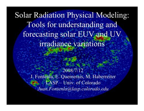
Solar Radiation Physical Modeling:Tools for understanding andforecasting solar EUV and UVirradiance variations2008/7/12J. Fontenla, E. Quemerais, M. HaberreiterLASP – Univ. of ColoradoJuan.Fontenla@lasp.colorado.edu

SRPM Project Goals•Diagnosis of physical conditions through thesolar atmosphere; energy balance of radiativelosses and mechanical heating.•Evaluating proposed physical processes todetermine the solar atmosphere structure andspectrum at all spatial and temporal scales.•Synthesizing solar irradiance spectrum andits variations to improve the above and producecomplete and quantitative physical models.•Forecasting spectral irradiance at any time andposition in the Heliosphere. Weekly and monthlyforecast is now becoming possible.

Layers of the solar atmosphere• Photosphere (using average 1D models and external 3D simulations)– Slow motions (few km/s) dominated by convection overshoot– Weak ionization– All particles are unmagnetized– Plasma beta > 1– At or near LTE• Chromosphere (using average 1D models and 3D MHD simulations)– Motions and inhomogeneities change from weak to strong– Weak ionization (n p

SRPM Flow Scheme0.8Carbon Ionization and Mass FLow......... Static case (w/dif)_____ Upflow case (w/dif)IonizationFraction0.60.40.20.010 4 2 3 4 5 6 7 8 9n lev ,n ion ,…(x,y,z,t)10 5 2 3 4 5 6 7 8 9Temperature (K)10 6IntermediateParametersEmittedSpectrumI(λ,µ,φ,t)Physical Models& ProcessesObservedSpectrumT,ne,nh,U,...(x,y,z,t)I(λ,µ,φ,t)

Photosphere (radiation/convection)Stein & Nordlund 2000 convection simulations snapshotsSRPM absolute radiance, wavelength and CLV dependenceC I 5381Mg I 4572CN band500 nm 800 nm 1200 nm 1600 nmSlit spectrum8000SRP M 306Stein & NordlundSRP M 306 * 0.95400Temperature (K)6000Height (km)20040000SRPM 306Stein & NordlundSRPM 306 + 30 km1 . 10 3 1 . 10 4 1 . 10 5 1 . 10 61 .10 3 1 .10 4 1 .10 5 1 .10 6Pressure (dyne cm^-2)Pressure (dyne cm^-2)Comparison of spatial averages with semi-empirical modelspoints to improvements in average models and in simulations

Solar Chromosphere(radiation/plasma heating)Discrete set of featuresassigned to variousheating levels.BDFUV (1540 A) continuumMDI magnetogramLog-normal distributionof heated areas in quietSun, probably due tosimilar distribution ofmagnetic features.LyαCa II K 3UV continuumRed cont.

Active Sun chromospheric featuresSunspot umbra and penumbrataken from continuum images,but plage and network pixelsfrom Ca II K data.Super-heated (plage) featuresin active regions are discretizedby two components.H P1Number of Pixels (relative to total)0.10.011 .10 31 .10 40.9 0.95 1 1.05 1.1 1.15Intensity (relative to median)

A set of models discretizes thedistribution of heated areas(other models for sunspot umbra &penumbra are not shown here)Upper chromosphere Lower chromosphere8000Temperature (K)60004000B 1001D 1002F 1003H 1004P 10050.1 1 10 100 1 .10 3 1 .10 4 1 .10 5Pressure (dyn cm^-2)Semi-empirical, in-pixel.NLTE radiative transfermodels built to account forthe radiance observations.

Transition region(radiation/conduction+diffusion+flows)Quiet Sunhva+ hvas, hda+hdas,h4Temperature (K)1 .10 6 Vernazza & Reeves data1 .10 51 .10 4Vernazza & Reeves dataDeere et alB 10011 .10 31.9 .10 8 1.95.10 8 2 .10 8 2.05.10 8 2.1 .10 8 2.15.10 8 2.2 .10 8Temperature (K)1 .10 6 AR Vernazza & Reeves data1 .10 51 . 10 4AR Vernazza & Reeves dataAR Deere et alH 10041 .10 31.82.10 8 1.83.10 8 1.84.10 8 1.85.10 8 1.86.10 8Height (cm)Height (cm)The low transition-region (T < 200,000 K) is strongly affectedby optically thick NLTE radiative transfer and particle diffusioneffects up to ~60,000 K. Above that the energy balance model isclose to the DEM standard curves for comparable abundances(note that SRPM uses abundances similar to Dere values).

Upper transition-regionTemperature (K)1 . 10 65 . 10 51.5 . 10 6 Vernazza & Reeves data2.5 .10 6Vernazza & Reeves dataDeere et alB 1011Temperature (K)2 .10 61.5 . 10 61 .10 65 .10 53 .10 6 AR Vernazza & Reeves dataAR Vernazza & Reeves dataAR Deere et alP 10152 .10 8 4 .10 8 6 .10 8 8 .10 8 1 .10 9 1.2 .10 9 1.4 .10 9Height (cm)5 .10 8 1 .10 9 1.5 .10 9Height (cm)Upper transition-region (T > 200,000 K) energy balance modelsare also close to the DEM ones with similar abundances. In theenergy balance models conduction dominates at the bottom butlocal energy dissipation becomes important at the top.

Corona and upper transition region(radiation+conduction+solar wind)QuietActiveTemperature (K)6 .10 6 Vernazza & Reeves dataDeere et alSRPM 10014 .10 62 . 10 6Temperature (K)6 . 10 6 AR Vernazza & Reeves dataAR Deere et alSRPM 10154 .10 62 .10 65 .10 9 1 .10 10 1.5 .10 10 2 .10 10 2.5 .10 105 .10 9 1 .10 10 1.5 .10 10 2 .10 10 2.5 .10 10Height (cm)Height (cm)The temperature reaches a maximum value (local energy dissipationis essential) and decreases again in the heliosphere. DEM cannothandle this behavior. Solar wind and coronal holes are features toconsider. In active regions, groups of hot loops are the key feature.

Tools for forecasting solar irradianceAssuming previous curve is bad Images of the near-side produce daily masks of featuresLy alpha irradiance0.00750.0070.0065Current rotationShifted previous rotation0.00610 20 30 40 50 60 70 80 90Days since 2005/8/1Using atmospheric models thespectrum is computed for any daySynoptic masks are refined by applying trendsNOAA 10808and far-side imaging:(far side)AR helioseismic image1 .10 7 CLog(T)6 CEFH540.01 0.1 1 10 100 1 .10 3 1 .10 4 1 .10 5Pressure (dyne cm^-2)Intensity (erg cm^-2 s^-1 sr^-1)1 .10 61 .10 51 .10 41 . 10 3EFH1215.5 1216WavelengthEARTHCourtesy of D. BraunWithout refinement thesynoptic mask featuresobsolescence makes it badAR backscattered imageNOAA 10808(near side)

EUV radiance spectra of solar featuresFeatures radiance spectraCombined QS radiance spectrumIntensity (mW m^-2 A^-1 sr^-1)1 .10 5 B 1001D 1002F 1003SUMER QS1 .10 41 .10 3100101Intensity (mW m^-2 A^-1 sr^-1)1 .10 5 SRPM QSSUMER QS1 .10 41 .10 31001010.1600 700 800 900 1000 1100 1200 1300 1400 1500 16000.1600 700 800 900 1000 1100 1200 1300 1400 1500 1600Wavelength (A)Wavelength (A)The models computed radiance matches the SOHO/SUMER spectraas the models were build for that. They provide other spectral rangesand extremely high resolution too. The QS combination of models(0.75 B+0.22 D+0.03 F) nearly matches the average QS in Curdt et al.atlas. (Preliminary spectra, work in progress..)

High resolution examplesChromosphericradiance exampleIntensity (mW m^-2 A^-1 sr^-1)600400200SRPM QSSUMER QS01455 1460 1465 1470 1475Wavelength (A)Irradiance (W m^-2 nm^-1)1 .10 3 100B 1001Rocket flight0.10.011 .10 31 . 10 41 .10 51 .10 61 .10 7101Low transition-regionirradiance example1 .10 850 52 54 56 58 60Wavelength (nm)In general there is good agreement on lines but individual linescan be off because of uncertainties in atomic data (mainlycollisional excitation rates). Also, so far we have not completedthe runs for the spectra of upper transition-region+coronal partsof the models which contribute many lines.

Preliminary Active RegionChromosphericLower transition-regionIntensity (erg s^-1 cm^-2 A^-1 sr^-1)1 .10 6 SRPM QSH 1004SUMER QSSUMER Plage1 .10 51 .10 41 .10 310010Intensity (erg s^-1 cm^-2 A^-1 sr^-1)1 .10 6 SRPM QS1 .10 5H 1004SUMER QSSUMER Plage1 .10 41 .10 31001011250 1300 1350 1400 1450 15001700 750 800 850 900 950 1000 1050 1100 1150 1200Wavelength (A)Wavelength (A)The UV chromospheric continuum matches fine inmodel P. However, improvement is needed in thelower transition-region of the active region models.