Components of nodal prices for electric power systems - Power ...

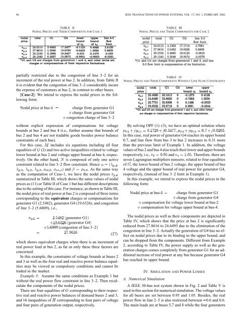
46 IEEE TRANSACTIONS ON POWER SYSTEMS, VOL. 17, NO. 1, FEBRUARY 2002TABLE IINODAL PRICES AND THEIR COMPONENTS FOR CASE 1TABLE IIINODAL PRICES AND THEIR COMPONENTS FOR CASE 2partially restricted due to the congestion of line 3–2 for anincrement of the real power at bus 2. In addition, from Table IIit is evident that the congestion of line 3–2 considerably incursthe expense of customers at bus 2, in contrast to other buses.[Case-2]: We intend to express the nodal prices in the followingform:TABLE IVNODAL PRICES AND THEIR COMPONENTS WITHOUT LINE FLOW CONSTRAINTSNodal price at bus-charge from generator G1charge from generator G4congestion charge of line 3–2without explicit expression of compensations for voltagebounds at bus 2 and bus 4 (i.e., further assume that bounds ofbus 2 and bus 4 are not tradable goods besides power balanceconstraints of each bus).For this case, includes six equations including all fourequalities of (2) and two active inequalities related to voltagelower bound at bus 2 and voltage upper bound at bus 4, respectively.On the other hand, is composed of only one activeconstraint related to line 3–2 flow constraint. Hence ,, , and - . As the same wayas the computation of Case-1, we have the nodal pricessummarized in Table III, which shows the same values of nodalprices as (11) or Table II of Case 1 but has different descriptionsdue to the setting of this case. For instance, as shown in Table III,the nodal price of real power at bus 2 is composed of three termscorresponding to the equivalent charges or compensations forgenerator G1 (2.5482), generator G4 (19.6326), and congestionof line 3–2 (5.6809), i.e.,generator G1generator G4congestion of line 3–2(27)which shows equivalent charges when there is an increment ofreal power load at bus 2, as far as only these three factors areconcerned.In this example, the constraints of voltage bounds at buses 2and 3 as well as the four real and reactive power balance equalitiesmay be viewed as compulsory conditions and cannot betraded in the market.Example 3: Assume the same conditions as Example 1 butwithout the real power flow constraint in line 3–2. Then recalculatethe components of the nodal prices.There are four equalities of corresponding to their respectivereal and reactive power balances of demand buses 2 and 3,and 16 inequalities of corresponding to four pairs of voltageand four pairs of generation output, respectively.By solving OPF (1)–(3), we have an optimal solution where, .In this case, real power of generator G4 reaches its upper bound0.7, and line flow from bus 3 to bus 2 increases to 0.31 morethan the previous limit of Example 1. In addition, the voltagevalues of bus 2 and bus 4 also reach their lower and upper boundsrespectively, i.e., and . Therefore, there areseven Lagrangian multipliers nonzero, related to four equalitiesof , the lower bound of bus 2 voltage, the upper bound of bus4 voltage and the upper bound of real power for generator G4,respectively, (instead of line 3–2 limit in Example 1).In this example, we intend to express the nodal prices in thefollowing form:Nodal price at bus- charge from generator G1charge from generator G4compensation for voltage lower bound at bus-2compensation for voltage upper bound at bus-4.The nodal prices as well as their components are depicted inTable IV, which shows that the price at bus 2 is significantlyreduced from 27.8616 to 24.6495 due to the elimination of thecongestion in line 3–2. Actually the generation of G4 has no effecton nodal prices due to its binding to the upper bound, andcan be dropped from the components. Different from Example2, according to Table IV, the power supply as well as the generationcharges comes completely from generator G1 for an additionalincrease of real power at any bus because generator G4has reached its upper bound.IV. SIMULATION AND POWER LOSSESA. Numerical SimulationA IEEE 30-bus test system shown in Fig. 2 and Table V isused in this section for numerical simulation. The voltage valuesfor all buses are set between 0.95 and 1.05. Besides, the realpower flow in line 2–5 is also restricted between 0.6 and 0.6.The main loads are at buses 5,7 and 8 while the four generators