Sustainable Withdrawal Rates for New Retirees in 2015

APPENDIX ON CAPITAL
MARKET ASSUMPTIONS
AND FEES
The capital market expectations connect the historical averages from Robert Shiller’s dataset together with the
current market values for inflation and interest rates. The equity premium is also muted for the first 10 years
to reflect the current PE value. This makes allowances for the fact that interest rates, inflation, and PE10 are
currently far from their historical averages, but it also respects historical averages and does not force returns to
remain low for the entire simulation.
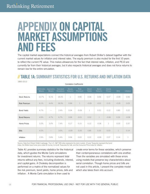
// TABLE 1A: SUMMARY STATISTICS FOR U.S. RETURNS AND INFLATION DATA
Table A1: SUMMARY STATISTICS FOR U.S. RETURNS AND INFLATION DATA
1890-2013
1890-2013
Correlation Coefficients
Arithmetic
Means
Geometric
Means
Standard
Deviations
Stocks
Returns
Risk
Premium
Bond
Yields
Bond
Returns
Home
Prices Bills Inflation
Stock Returns
10.7%
9.1%
18.3%
1
0.99
0.04
0.06
0.17
-0.09
0.06
Risk Premium
6.1%
4.4%
18.3%
0.99
1
-0.09
-0.01
0.15
-0.20
0.03
Bond Yields
4.7%
---
2.4%
0.04
-0.09
1
0.52
0.12
0.85
0.22
Bond Returns
4.9%
4.7%
6.7%
0.06
-0.01
0.52
1
-0.06
0.33
-0.09
Home Prices
3.3%
3.0%
7.4%
0.17
0.15
0.12
-0.06
1
0.03
0.37
Bills
4.5%
---
3.0%
-0.09
-0.20
0.85
0.33
0.03
1
0.14
Inflation
2.9%
2.8%
5.4%
0.06
0.03
0.22
-0.09
0.37
0.14
1
Source: Data from Robert Shiller’s webpage. The U.S. S&P 500 index represents the stock market, 10-year Treasuries represent the bond
index, the Shiller-Case home price index for homes, 6-month Treasuries for bills, and the Consumer Price Index for inflation.
Table A1 provides summary statistics for the historical
data, which guides the Monte Carlo simulations
for investment returns. The returns represent total
returns without any fees, including dividends, interest,
and capital gains. A Cholesky decomposition is
performed on a matrix of the normalized values for
the risk premium, bond yields, home prices, bills and
inflation. A Monte Carlo simulation is then used to
create error terms for these variables, which preserve
their contemporaneous correlations with one another.
Then the variables are simulated with these errors
using models that preserve key characteristics about
serial correlation. Though home prices and bills are
not used in this article, I present the complete model
which also takes them into account.
13 FOR FINANCIAL PROFESSIONAL USE ONLY - NOT FOR USE WITH THE GENERAL PUBLIC