Laplace transform isotherm .pdf - University of Hertfordshire ...

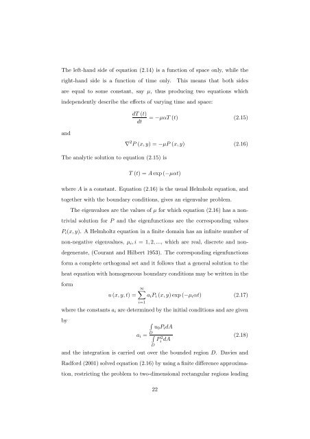
The left-hand side of equation (2.14) is a function of space only, while the
right-hand side is a function of time only. This means that both sides
are equal to some constant, say µ, thus producing two equations which
independently describe the effects of varying time and space:
and
dT (t)
dt
The analytic solution to equation (2.15) is
= −µαT (t) (2.15)
∇ 2 P (x,y) = −µP (x,y) (2.16)
T (t) = Aexp (−µαt)
where A is a constant. Equation (2.16) is the usual Helmholz equation, and
together with the boundary conditions, gives an eigenvalue problem.
The eigenvalues are the values of µ for which equation (2.16) has a non-
trivial solution for P and the eigenfunctions are the corresponding values
Pi(x,y). A Helmholtz equation in a finite domain has an infinite number of
non-negative eigenvalues, µi,i = 1,2,..., which are real, discrete and non-
degenerate, (Courant and Hilbert 1953). The corresponding eigenfunctions
form a complete orthogonal set and it follows that a general solution to the
heat equation with homogeneous boundary conditions may be written in the
form
u(x,y,t) =
∞�
aiPi (x,y) exp (−µiαt) (2.17)
i=1
where the constants ai are determined by the initial conditions and are given
by
�
u0PidA
D
ai = �
D
P 2
i dA
(2.18)
and the integration is carried out over the bounded region D. Davies and
Radford (2001) solved equation (2.16) by using a finite difference approxima-
tion, restricting the problem to two-dimensional rectangular regions leading
22