Stochastic Evaluation of Exploration Assets - MEIVAE

Medardo Yañez, Karina Semeco, Michele Leccese, Pedro Gil, José Fariñas, Miguel Agüero. 5
applying Bayes Theorem [1], [2], [15] in its meaning to the
treatment of conditional probabilities, the probability of finding a
certain prospect "X”, is expressed as:
P(X)=P(S) x P(X|S) (5)
Table 1 shows the estimation of the individual probabilities P (X)
for the example of 5 prospects.
Probabilistic Factors
Prospect A Pospecto B Prospect C Prospect D Prospect E
P1a Reservoir Facies 0.8 0.8 0.8 0.8 0.8
P1b Porosity 0.6 1.0 0.5 0.8 0.9
P2a Trap Identification 1.0 0.9 0.9 0.7 0.6
P2b Seal 0.9 0.9 0.8 1.0 1.0
P3a Mature Sorce Rock 0.7 0.7 0.7 0.7 0.7
P3b Migration 1.0 0.8 0.9 0.8 0.8
P4 Retention 1.0 1.0 1.0 1.0 1.0
P (B|Ā) = [0.3639 x (1 – 0.54)] / (1 – 0.3024) = 0.239
Probability of Prospect C being successful given that A was a
failure:
P (C|Ā) = [0.1814 x (1 – 0.54)] / (1 – 0.3024) = 0.120
Probability of Prospect D being successful given that A was a
failure:
P (D|Ā) = [0.2509 x (1 – 0.54)] / (1 – 0.3024) = 0.165
Probability of Prospect E being successful given that A was a
failure:
P (E|Ā) = [0.2419 x (1 – 0.54)] / (1 – 0.3024] = 0.160
P(S)=P1a x P3a x P4 Common Factors 0.56 0.56 0.56 0.56 0.56
P(X/S)=P1b x P2a x P2b x P3b Independent Factors 0.54 0.648 0.324 0.448 0.432
P(X)=P(S) x P(X/S) Individuial Probability 0.3024 0.3629 0.1814 0.2509 0.2419
A
Failure
(Dry)
P(A)
1-P(A)=0.698
1
0.698
Table 1 - Shows factors P1a, P3a and P4 common for five
prospects, and P1b, P2a, P2b and P3b, uncommon or
independent for the 5 prospects. This is calculated by P (S) = P1a
x P3a x P4, and P (X / S) = P1b x P2a x P2b x P3b, for each
prospect, to finally obtain the individual probabilities P (A), P (B ),
P (C), P (D) and P (E) using the equation of Bayes P (x) = P (S) x
P (x / S).
B
C
Discovery
Failure
Discovery
Failure
P(B P(B/A)=0.648
/
0.239
(1-P(B/A))=0.352
/
0.761
P(C P(C/A)=0.324
/
0.120
(1-P(C/A))=0.676
/
0.880
With the results summarized in Table 1, now it can be estimated
how the individual probabilities are affected, for example in the
case of success of Prospect A, using the tree shown in Figure 3.
D
Discovery
Failure
P(D P(D/A)=0.448
/
0.165
(1-P(D/A))=0.552
/
0.835
E
Discovery
Failure
P(E P(E/A)=0.432
/
0.160
(1-P(E/A))=0.568
/
0.840
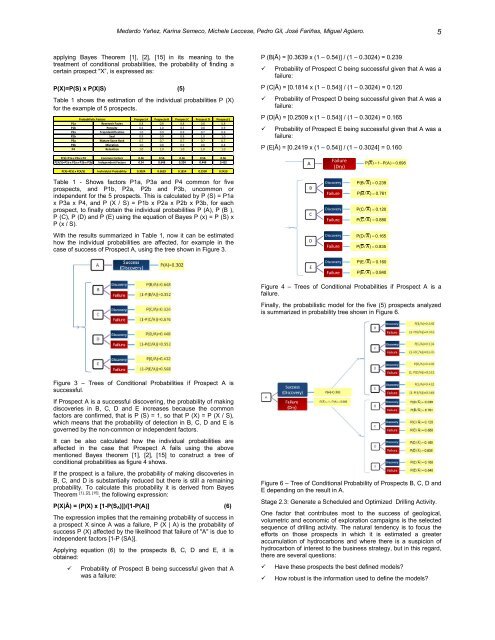
Figure 4 – Trees of Conditional Probabilities if Prospect A is a
failure.
Finally, the probabilistic model for the five (5) prospects analyzed
is summarized in probability tree shown in Figure 6.
Figure 3 – Trees of Conditional Probabilities if Prospect A is
successful.
If Prospect A is a successful discovering, the probability of making
discoveries in B, C, D and E increases because the common
factors are confirmed, that is P (S) = 1, so that P (X) = P (X / S),
which means that the probability of detection in B, C, D and E is
governed by the non-common or independent factors.
It can be also calculated how the individual probabilities are
affected in the case that Prospect A fails using the above
mentioned Bayes theorem [1], [2], [15] to construct a tree of
conditional probabilities as figure 4 shows.
If the prospect is a failure, the probability of making discoveries in
B, C, and D is substantially reduced but there is still a remaining
probability. To calculate this probability it is derived from Bayes
Theorem [1], [2], [15] , the following expression:
P(X|Ā) = (P(X) x [1-P(S A)])/[1-P(A)] (6)
The expression implies that the remaining probability of success in
a prospect X since A was a failure, P (X | A) is the probability of
success P (X) affected by the likelihood that failure of "A" is due to
independent factors [1-P (SA)].
Applying equation (6) to the prospects B, C, D and E, it is
obtained:
Probability of Prospect B being successful given that A
was a failure:
Figure 6 – Tree of Conditional Probability of Prospects B, C, D and
E depending on the result in A.
Stage 2.3: Generate a Scheduled and Optimized Drilling Activity.
One factor that contributes most to the success of geological,
volumetric and economic of exploration campaigns is the selected
sequence of drilling activity. The natural tendency is to focus the
efforts on those prospects in which it is estimated a greater
accumulation of hydrocarbons and where there is a suspicion of
hydrocarbon of interest to the business strategy, but in this regard,
there are several questions:
Have these prospects the best defined models?
How robust is the information used to define the models?