The path length of random skip lists - Institut für Analysis und ...
The path length of random skip lists - Institut für Analysis und ...
The path length of random skip lists - Institut für Analysis und ...

Create successful ePaper yourself
Turn your PDF publications into a flip-book with our unique Google optimized e-Paper software.
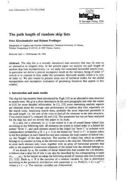
Acta Informatica 31, 775-792 (1994)<br />
<strong>The</strong> <strong>path</strong> <strong>length</strong> <strong>of</strong> <strong>random</strong> <strong>skip</strong> <strong>lists</strong><br />
Peter Kirschenh<strong>of</strong>er and Helmut Prodinger<br />
Department <strong>of</strong> Algebra and Discrete Mathematics, Technical University <strong>of</strong> Vienna,<br />
Wiedner Hauptstrasse 8-10/118, A-1040 Vienna, Austria<br />
Received April 1, 1993/January 28, 1994<br />
Abstract. <strong>The</strong> <strong>skip</strong> list is a recently introduced data structure that may be seen as<br />
an alternative to (digital) tries . In the present paper we analyze the <strong>path</strong> <strong>length</strong> <strong>of</strong><br />
<strong>random</strong> <strong>skip</strong> <strong>lists</strong> asymptotically, i .e . we study the cumulated successful search costs .<br />
In particular we derive a precise asymptotic result on the variance, being <strong>of</strong> order n 2<br />
(which is in contrast to tries <strong>und</strong>er the symmetric Bernoulli model, where it is only<br />
<strong>of</strong> order n) . We also intend to present some sort <strong>of</strong> technical toolkit for the skilful<br />
manipulation and asymptotic evaluation <strong>of</strong> generating functions that appear in this<br />
context .<br />
1 . Introduction and main results<br />
11,<br />
INfoFmaUca "<br />
© Springer-Verlag 1994<br />
<strong>The</strong> <strong>skip</strong> list has recently been introduced by Pugh [15] as an alternative data structure<br />
to search trees . We give a short description in the next paragraphs and refer the reader<br />
to [13] for more detailed information . In [1], [13] some interesting analytic aspects<br />
are obtained about the average case performance <strong>of</strong> <strong>random</strong> <strong>skip</strong> <strong>lists</strong>, especially on<br />
the search costs . Analyzing search trees, probably the most important parameter is<br />
the <strong>path</strong> <strong>length</strong>, i .e . the sum <strong>of</strong> the costs to find all the elements in the data structure,<br />
("successful search"), compare [4] and [12] . This parameter has not yet been analyzed<br />
for the <strong>skip</strong> list, and we devote this paper to its study .<br />
In a <strong>skip</strong> list n elements (n > 1) are stored in a set <strong>of</strong> sorted linear linked <strong>lists</strong><br />
according to the following rule : all elements are stored in sorted order in a linked list<br />
named "level I", and each element stored in the linked list "level i" is included with<br />
(independent) probability q (0 < q < 1) in the linked list "level i + 1" . A header refers<br />
to the first element in each linked list and also contains the total number <strong>of</strong> linked <strong>lists</strong>,<br />
i .e . the "height" <strong>of</strong> the data structure . <strong>The</strong> number <strong>of</strong> linked <strong>lists</strong> which an element<br />
belongs to is constant as long as the element exists in the <strong>skip</strong> list . <strong>The</strong>refore it suffices<br />
to store each element only once, together with an array <strong>of</strong> horizontal pointers that<br />
refer to the respective consecutive elements <strong>of</strong> the linked <strong>lists</strong> the element belongs to .<br />
If we denote by ai the number <strong>of</strong> linear linked <strong>lists</strong> that contain the i-th element,<br />
it follows that a <strong>skip</strong> list <strong>of</strong> size n can also be described by the corresponding n-tuple<br />
(a,, . . . , an ) . In the sequel we adopt the following model <strong>of</strong> <strong>random</strong> <strong>skip</strong> <strong>lists</strong> (compare<br />
[1], [13]) . Each ai E N is the outcome <strong>of</strong> a <strong>random</strong> variable Gi that is distributed<br />
according to the geometric distribution with parameter p, i .e. Prob{Gi = k} = pqk-I ,<br />
where q = I - p. <strong>The</strong> <strong>random</strong> variables are independent .
<strong>The</strong> reader is warned that in the earlier papers the roles <strong>of</strong> p and q are interchanged .<br />
Nevertheless, we find it easier to stay with the present notation that is classical in the<br />
context <strong>of</strong> the geometric distribution .<br />
<strong>The</strong> search for the i-th element starts at the header <strong>of</strong> the top level linked list.<br />
This list is followed until the index <strong>of</strong> the next element in the list is greater or equal<br />
to i (or the reference is null) . In this instance the search continues one level below .<br />
<strong>The</strong> search terminates at level I with an equality test as the last comparison .<br />
In the figure below we depict the search <strong>path</strong> for the 4-th element in a <strong>random</strong><br />
<strong>skip</strong> list <strong>of</strong> size 4 .<br />
In<br />
51<br />
93<br />
1]<br />
V<br />
∎<br />
header 2' 3" 4 0.<br />
Following [13] we define the search cost for the i-th element as the number <strong>of</strong><br />
pointer expections excluding the last one for the equality test (i .e . 13 in the example<br />
above) . Each instance <strong>of</strong> a pointer inspection is marked by a dot in the figure . Observe<br />
that the last pointer expection comes up with the third element at level 1 . <strong>The</strong> search<br />
cost may be split up into the sum <strong>of</strong> a "vertical cost" corresponding to pointer inspections<br />
<strong>of</strong> pointers refering to elements at a position > i (that initiate the continuation <strong>of</strong><br />
the search one level below, 11 in the example) and a "horizontal cost" corresponding<br />
to the remaining pointer inspections, i .e . the number <strong>of</strong> horizontal steps on the <strong>path</strong><br />
from the header to the i-th element (2 in the example) . We define the horizontal <strong>path</strong><br />
<strong>length</strong> X, = Xn (p) <strong>of</strong> a <strong>skip</strong> list p containing n elements as the sum <strong>of</strong> the horizontal<br />
search costs <strong>of</strong> all elements in p . <strong>The</strong> vertical <strong>path</strong> <strong>length</strong> Yn = Yn (p) is defined<br />
analogously . Finally, the total <strong>path</strong> <strong>length</strong> or total cost Cn is X, + Yn . X n , Yn and<br />
Cn are <strong>random</strong> variables <strong>und</strong>er the above defined probability model for <strong>random</strong> <strong>skip</strong><br />
<strong>lists</strong> .<br />
It is an easy observation that the vertical search cost for each element equals<br />
the height <strong>of</strong> the <strong>skip</strong> list, so that Yn (p) is n times the height <strong>of</strong> p . <strong>The</strong> horizontal<br />
search cost is more intricate . Let us return to our alternative description <strong>of</strong> the <strong>skip</strong><br />
<strong>lists</strong> as n-tuples (a, , . . . , a n ) from above . <strong>The</strong> height clearly equals the maximum <strong>of</strong><br />
(a,, . , a n ) . <strong>The</strong> horizontal search cost is zero for the first element . Let now i > 2 .<br />
If we follow the <strong>path</strong> from the header to the i - 1-th element in reverse order we find<br />
that for the i-th element the horizontal cost is the number <strong>of</strong> right-to-left maxima in<br />
(a,, . . . , aa_, ), i .e. the number <strong>of</strong> elements a j (1 _< j < i - 1) that are larger than or<br />
equal to aj , aj + ,, . . . , ati_ 1 . (Observe that the convention to call a1_ 1 itself a rightto-left<br />
maximum ensures that the horizontal step connecting the <strong>path</strong> with the header<br />
is counted, too .) We may conclude that the horizontal <strong>path</strong> <strong>length</strong> <strong>of</strong> (a], . . , a n ) is<br />
the sum <strong>of</strong> the numbers <strong>of</strong> right-to-left maxima <strong>of</strong> the sequences a, , . . . , ai_ 1 for<br />
2
<strong>The</strong> <strong>path</strong> <strong>length</strong> <strong>of</strong> <strong>random</strong> <strong>skip</strong> <strong>lists</strong> 7 7 7<br />
With respect to expectations, the horizontal <strong>path</strong> <strong>length</strong> is simply the sum <strong>of</strong> all<br />
the horizontal search costs . This is also easy to check, comparing [14, Lemma 2] and<br />
our formula (2 .7) . However, with respect to variances the parameters are different,<br />
and the <strong>path</strong> <strong>length</strong> has proved to be more interesting . (For tries, Patricia tries and<br />
digital search trees, these analyses are quite challenging and are to be fo<strong>und</strong> in [7],<br />
[8], [9] .) <strong>The</strong> results about the variance <strong>of</strong> the horizontal <strong>path</strong> <strong>length</strong> Xn and <strong>of</strong> the<br />
total cost Cn are thus considered to be our main findings in the present paper . We<br />
also intend to present some sort <strong>of</strong> technical toolkit for the manipulation <strong>of</strong> generating<br />
functions that will frequently occur with the analysis <strong>of</strong> <strong>skip</strong> list parameters .<br />
In the following we summarize our main results . Here and in the whole paper,<br />
we will use the handy abbreviations Q = q -I and L = log Q .<br />
For the sake <strong>of</strong> completeness we start with a formulation <strong>of</strong> the asymptotics <strong>of</strong><br />
the expectations . Observe that these estimates can also be computed from the results<br />
<strong>of</strong> [13] on the search cost <strong>of</strong> specified elements, though the notion <strong>of</strong> <strong>path</strong> <strong>length</strong> is<br />
not considered there . (iii) is equivalent to [13, <strong>The</strong>orem 4] .<br />
Proposition 1 . (i) <strong>The</strong> expected value E(X,) <strong>of</strong> the horizontal <strong>path</strong> <strong>length</strong> in a <strong>random</strong><br />
<strong>skip</strong> list containing n elements fulfills for n --> oo<br />
- 1<br />
E(X,,,) = (Q - 1)n (logQ n + 'Y L - 1 2 + 1 L 6 1 (logQ n)) + O(log n)<br />
where -y is Euler's constant and 61(x) _ T (-1 - 2 7 i )e2k-7rix is a continuous<br />
kg0<br />
periodic function <strong>of</strong> period 1 and mean zero . (T is the Gamma-function .)<br />
(ii) <strong>The</strong> expected value <strong>of</strong> the vertical <strong>path</strong> <strong>length</strong> fulfills for n -* oo<br />
where 62(x) _<br />
7<br />
E(Y,~) = n logQ n + n ( L + 1 2 - 1L62(logQ n)) + O(log n),<br />
kq0<br />
2kLi) e 2knix .<br />
L<br />
(iii) <strong>The</strong> expected value E(Cn ) <strong>of</strong> the total cost fulfills for n --* oo<br />
E(Cn ) = Qn logQ n + Ti ( (7<br />
where 6 3 (x) = 6 1 (x) - 62 (x) .<br />
1 +1<br />
L<br />
- 2 +1+ L 63 (logQ n)) + O(log n)<br />
Remark. As a consequence <strong>of</strong> the exponential decrease <strong>of</strong> the r-function along vertical<br />
lines (compare (2 .37)) we have that the amplitude <strong>of</strong> the functions bi(x) here and in<br />
the sequel is very small for all reasonable values <strong>of</strong> q, e .g . 0 .1 < q < 0 .9 .<br />
<strong>The</strong> asymptotic equivalents for the second moments <strong>of</strong> the <strong>path</strong> <strong>length</strong>s are given<br />
in the sequel, and the two corresponding theorems are the main results <strong>of</strong> this paper .<br />
<strong>The</strong>orem 1 . <strong>The</strong> variance Var(Xn ) <strong>of</strong> the horizontal <strong>path</strong> <strong>length</strong> in a <strong>random</strong> <strong>skip</strong> list<br />
containing n elements fulfills for n -; oo<br />
Var X<br />
2 2 Q+ 1 1 7r 2 87r2 2<br />
( ) = (Q - 1) n<br />
+O n l+E<br />
) I E>o,<br />
2(Q - 1)L + L 2 6L 2 + L2 h(" L ) - c + b a (logQ n)
where<br />
where<br />
a2 =<br />
h(x) =<br />
Finally the following theorem holds .<br />
e k x<br />
)2 ,<br />
-1<br />
~ 1<br />
aI = L k> 1 k(L 2 + 4k 2 7r 2 ) sinh(2k7r 2/L)<br />
and 84(x) is again continuous, periodic <strong>of</strong> period I and mean zero .<br />
With regard to the vertical <strong>path</strong> <strong>length</strong>, i .e . n times the maximum element, we<br />
have from [5] or [17]<br />
2<br />
Var(Yn ) = - a2 + 85(logQ n) + O(n<br />
I+E ),<br />
n2 6L2 + 12<br />
<strong>The</strong>orem 2 . (i) <strong>The</strong> covariance Cov(X n , Yn ) <strong>of</strong> the horizontal and the vertical <strong>path</strong><br />
<strong>length</strong>s in a <strong>random</strong> <strong>skip</strong> list containing n elements fulfills for n --+ oo<br />
1 7r 2 2 2<br />
Cov(Xn , Y,.,) _ (Q - 1)n 2 { L2 6L2 + L2 h ( 4L ) - a + L<br />
with h and a1 from <strong>The</strong>orem 1 .<br />
k<br />
- 1)<br />
2<br />
+ 86(log Q n) + O(n<br />
I+E ),<br />
(ii) <strong>The</strong> variance Var(Cn ) <strong>of</strong> the total cost fulfills for n --~ oo<br />
2 2 2<br />
Var(Cn ) _ (Q 2 - 1) n2 2L + L 2 6L2 + L 2 h ( 4L )<br />
- a 1<br />
+ 2(Q - 1)n<br />
2{ 1 1 k<br />
L k>1 Qk - 1 k i (Q k - 1) 2<br />
+ n2<br />
2<br />
6L2 + - a2 + 87 (logQ n)<br />
12<br />
+E<br />
+ O(nl<br />
)<br />
k>I<br />
Qk 1- 1<br />
<strong>The</strong>orems I and 2 show that the variances <strong>of</strong> the <strong>path</strong> <strong>length</strong>s are <strong>of</strong> order n 2 ,<br />
whereas the variances <strong>of</strong> the corresponding parameter for regular symmetric tries<br />
(<strong>und</strong>er the Bernoulli model or the Poisson model) are <strong>of</strong> order n . This means that<br />
<strong>random</strong> <strong>skip</strong> list parameters are not as closely concentrated aro<strong>und</strong> their expectations<br />
as the corresponding parameters for tries .<br />
It is interesting to investigate the leading term <strong>of</strong> the variance <strong>of</strong> the total cost<br />
(<strong>The</strong>orem 2 (ii)) for different values <strong>of</strong> q (resp . Q = q -1 ) numerically . It turns out<br />
that the constant K in Var(Cn ) n 2 (K + 87(logQ n)) takes its minimum value for<br />
q = 0 .31 . . ., which differs a little from q = e = 0 .36 . . ., where the main term <strong>of</strong>
q<br />
0 .1<br />
0 .2<br />
0 .3<br />
0.31 . . .<br />
0 .4<br />
0 .5<br />
0 .6<br />
0 .7<br />
0 .8<br />
0 .9<br />
K<br />
10 .57 . . .<br />
3 .16 . . .<br />
2 .15 . . .<br />
2.13 . . .<br />
2 .44 . . .<br />
3 .66 . . .<br />
6 .41 . . .<br />
12 .96 . . .<br />
33 .03 . . .<br />
149 .35 . . .<br />
the expectation takes its minimum . Nevertheless we can conclude that for values <strong>of</strong><br />
q close to e, the variance is close to its minimum, too . Below we give a small table<br />
<strong>of</strong> q = Q- ' and the corresponding values <strong>of</strong> the constant K .<br />
<strong>The</strong> pro<strong>of</strong> <strong>of</strong> the theorems is given in the next two sections . Section 2 contains the<br />
considerations on the horizontal <strong>path</strong> <strong>length</strong> . It starts with a set-up <strong>of</strong> the appropriate<br />
generating functions, presents a transformation that allows to express the coefficients<br />
as complex contour integrals in a very efficient manner, and finally reveals the asymptotic<br />
equivalents <strong>of</strong> the expectation and the second moment as the sums <strong>of</strong> residues at<br />
certain poles . Section 3 contains the technical details concerning the second moment<br />
<strong>of</strong> the total cost . In Sect . 4 we present an alternative representation for the constants<br />
in the leading terms <strong>of</strong> <strong>The</strong>orems 1 and 2 which is better suited for numerical evaluations<br />
if q is close to 0 . For this purpose a series transformation result has to be proved<br />
that is <strong>of</strong> its own interest . In the final Sect . 5 we add some results on parameters that<br />
can be analyzed using the same toolkit as prepared for the analysis <strong>of</strong> the <strong>path</strong> <strong>length</strong> .<br />
2 . <strong>The</strong> horizontal <strong>path</strong> <strong>length</strong><br />
We start from the interpretation <strong>of</strong> a <strong>skip</strong> list p <strong>of</strong> size n + 1 as a finite sequence<br />
(a,, . . . , an+ ,), n > 0, ai E {1, 2, 3 . . . . } . <strong>The</strong> horizontal <strong>path</strong> <strong>length</strong> Xn,+,( p) is the<br />
sum b(p) <strong>of</strong> all numbers <strong>of</strong> right-to-left maxima in the subsequences (a,, . . . , a 2 ),<br />
I < i < n, <strong>of</strong> p' = (a, , . . . , a n ) . In order to obtain an expression for the corresponding<br />
probability generating function it is convenient to start from the following<br />
combinatorial decomposition :<br />
Let m be the maximal element occuring in p' . <strong>The</strong>n we can write p' in a unique<br />
way as<br />
p=amr, where a E {1, . . .,m- l} 1r E {1, . . .,m} (2 .1)<br />
(fixing the leftmost occurence <strong>of</strong> the maximum m) . From this decomposition it follows<br />
that<br />
b(p') = b(amT) = b(a) + b(-r) + 1irI + l, b(E) = 0, (2 .2)<br />
since the contribution <strong>of</strong> the leftmost maximum is 1 plus the number <strong>of</strong> the succeding<br />
elements . <strong>The</strong> reader might observe that relation (2 .2), in the context <strong>of</strong> permutations<br />
p' (and thus binary search trees), describes the right-sided <strong>path</strong> <strong>length</strong> . However the<br />
probabilistic models are quite different . (Compare e .g . [101, [16] .)
We introduce the bivariate generating functions P-'(z, y), where the coefficient<br />
<strong>of</strong> z"y 3 is the probability that a <strong>skip</strong> list p with n+ 1 elements has maximum element<br />
(<strong>of</strong> the prefix p') m and horizontal <strong>path</strong> <strong>length</strong> j (<strong>of</strong> p) . P5 m (z, y) and P
<strong>The</strong> <strong>path</strong> <strong>length</strong> <strong>of</strong> <strong>random</strong> <strong>skip</strong> <strong>lists</strong> 781<br />
In this way we find<br />
H < ' (z) - H
E(Xn) Q<br />
1: ( k ) (-1) k Qk_ 1<br />
k=2<br />
In order to get the asymptotic equivalent for E(X n ) we might apply a Mellin transform<br />
approach (cf . [4]) to (2 .7) . Alternatively, the expression (2 .8) can be rewritten<br />
as a complex contour integral (Rice's method), namely<br />
E(X",) = q • 2~ri<br />
1<br />
-<br />
1<br />
B(n + 1, -z) Qz _~ -1dz , (2 .9)<br />
where B(x, y) = r(x)r(y) is the Beta function and the contour C encircles the poles<br />
r(x+y)<br />
z = 2, 3, . . . , n . Now the asymptotics are obtained by extending the contour C "to the<br />
left" and collecting the additional residues . (Compare [3] for technical details <strong>of</strong> this<br />
procedure .)<br />
In the integral (2 .9) we have additional poles with real part larger than zero at<br />
z = Xk, Xk = jogQ , k E Z . <strong>The</strong> computation <strong>of</strong> the residues is standard and can be<br />
performed e .g . by MAPLE . It yields for the double pole z = 1<br />
Res z =, B(n + 1, -z)<br />
1<br />
QZ-t<br />
-<br />
L)<br />
1 = Ln (Hn-1 - 1 - 2 ,<br />
(2 .8)<br />
with L = log Q and Hn the n-th Harmonic number, and thus the asymptotic contribution<br />
to E(Xn )<br />
P L ( log n + 7 - I - 2) + O(log n) .<br />
Similarly the simple poles z = 1 + Xk, k ' 0, contribute<br />
q L E T(-1 - Xk)n'+xk (1 +O(n)) . (2 .10)<br />
kq0<br />
Collecting all contributions we have Proposition 1 (i) .<br />
In the sequel we concentrate on our main goal, namely the computation <strong>of</strong> the<br />
variance Var(Xn ) . We have<br />
Var(X n ) = [zn- ' ]H(z) + E(Xn ) - E(Xn ) 2 , (2.11)<br />
so that we need a well suited expression for the coefficients <strong>of</strong> H(z) .<br />
For this purpose it is extremely useful to start with the following technical observations<br />
. In [2] Flajolet and Richmond made extensive use <strong>of</strong> the relation<br />
A (z) _ an z n ~---~<br />
1-<br />
1<br />
w<br />
A (<br />
1-<br />
n>O<br />
WW)<br />
Of course this relation can be inverted to read<br />
= (k) ak . (2 .12)<br />
wn<br />
n>o k=O<br />
1<br />
A(z) - ( k ) (- 1) k f (k)) zn ~--~ 1 - w A (w -<br />
n>0 k=o<br />
n>O<br />
f(n)wn . (2 .13)<br />
<strong>The</strong> alternating sum can now be rewritten by Rice's method (compare above), and in<br />
this way we find
Lemma 1 . Let A(z) be a formal power series and<br />
with fo = f1 = . . . =f,-, =0. <strong>The</strong>n<br />
fn = [w 12 ) 1 AC w ~, n > 0 (2 .14)<br />
1-w w-1<br />
[z n]A(z) = 2ri j<br />
C(s, . . .,n)<br />
B(n + 1, -z) f (z)dz, (2 .15)<br />
where C(s, . . . , n) encircles the poles z = s, s + 1, . . . , n, B is the Beta function and<br />
f (z) is analytic inside C with f (n) = fn for all n > s .<br />
<strong>The</strong> following generalization will be useful .<br />
Lemma 2 . With the assumptions <strong>of</strong> Lemma I we have<br />
Pro<strong>of</strong>. With z = w' 1 we have (1 - z) -r = (- 1) r Z, , so that<br />
[z 12 ](1 - z) - ' A(z) _ (-1)r[zn+r)wTA(z) .<br />
<strong>The</strong> result follows now from Lemma 1 . 0<br />
In order to compute the coefficients fn in (2 .14) for the formal series A(z) occuring<br />
in our problem we will frequently apply<br />
Lemma 3 . Let C and D be formal power series . <strong>The</strong>n<br />
and<br />
[zn)<br />
1 r A(z) = (-1)<br />
(1 - z) 27ri<br />
]<br />
i>1<br />
[w n ]<br />
i>O<br />
i>I<br />
C(wg z ) Qn l- 1 [wn]C(w), n > 1, (2 .18)<br />
I<br />
Qn _<br />
n<br />
m=1<br />
I<br />
[w m)C(w) . _ gm<br />
[w'-m)D(w), (2 .20)<br />
C(wgt)D(wqj)<br />
I 1, (2<br />
2 .19)<br />
1) [wn]C(w),<br />
-<br />
C(wq`)D(wg3 )<br />
Pro<strong>of</strong>. Immediate. D<br />
Now we are ready to express [zn -1 ]H(z) as a complex contour integral . We confine<br />
ourselves here to show how the method works for two <strong>of</strong> the seven terms in (2 .6) .<br />
Let us start with the relatively simple first one, namely<br />
A 1 (z) _ ( 1 z )<br />
With the substitution z = w"' I we have<br />
and therefore<br />
From Lemma 3 (2 .18) we find<br />
<strong>The</strong>refore, by Lemma 2,<br />
Here we have<br />
where<br />
A 7 (z)<br />
1 A7<br />
1 -w Cw- 1/<br />
i>1<br />
i<br />
:<br />
Qq12<br />
=<br />
( l I<br />
Z)2 A1(z) .<br />
1 _ l -w<br />
Qi] 1 - wgti<br />
1 1wA1Cww 1) =-<br />
[zn-1 ]A1(z) = 2i 1 B(n + 2, -z) Q Z 2 21 dz . (2 .24)<br />
(1 -<br />
w l E S
-1 w S< 1(w)S
With a = Em>1 Q ,"- 1 .<br />
In order to get the asymptotic behaviour <strong>of</strong> [z'- ' ]H(z) for n oo we extend<br />
the contour <strong>of</strong> integration to a large rectangle and shift the left side to the line<br />
Re z = 1 + E, E > 0. <strong>The</strong>n [z" -1 ]H(z) equals the sum <strong>of</strong> residues at the additional<br />
poles included in the contour with an error term <strong>of</strong> order O(n 1+ E) (compare (3] for<br />
technical details <strong>of</strong> the estimate <strong>of</strong> the error term) . In our instance the additional<br />
poles originate from the second integral, and they are located at z = 2 (triple) resp .<br />
z = 2 + Xk, k E Z \ {0} (simple) . <strong>The</strong> computation <strong>of</strong> the residues can be performed<br />
by hand, or, more preferably, e .g . by Maple, and we find for the residue at z = 2<br />
2(Q - 1)2<br />
+ Hn2) 1<br />
n + 1 ~H,2,_i Hn<br />
1 (1 + 2<br />
2 L 2 L2 L )<br />
+ 3 + L2 - 2(a +,3) + 2L + (Q 1 I )L }'<br />
(2 .31)<br />
where L = log Q, H,,, resp . H(,,,2) are the harmonic numbers <strong>of</strong> first resp . second order,<br />
and ,0= E 1 2 .<br />
m>1<br />
(Qm- 1 )<br />
<strong>The</strong> asymptotic equivalent <strong>of</strong> (2 .31) is<br />
2 g 2<br />
2(Q - 1) 2 n12 Q n + n 2 logQ<br />
n C L 2 L l<br />
2 1 1 'Y 'Y 'Y2<br />
~2<br />
1 1 l<br />
+n (6+L2-a-~-2L L2+ 2L2+ 12L2+ 4L + 2(Q - IL) )<br />
+O (n log e n)<br />
. (2.32)<br />
I<br />
<strong>The</strong> first order poles at z = 2 + Xk, k E Z \ {0}, give a contribution <strong>of</strong> the form<br />
n 2 68 (log Q n) + 0(n), (2 .33)<br />
where 58(x) is a continuous periodic function <strong>of</strong> period 1 and mean zero . <strong>The</strong> Fourier<br />
coefficients <strong>of</strong> 68(x) can be obtained explicitly from the residues at the above . mentioned<br />
poles . <strong>The</strong>y can be used to show that the amplitude <strong>of</strong> 68(x) is very small<br />
(because <strong>of</strong> the exponential decrease <strong>of</strong> the F-function along . vertical lines) . Since<br />
from the practical .point <strong>of</strong> view 6 8 (x) has almost no influence on the variance, we<br />
omit these calculations here .<br />
Combining (2 .32), (2 .33) and Proposition 1 we get the asymptotic equivalent <strong>of</strong><br />
Var(Xn,) according to (2 .11) . <strong>The</strong> reader should take notice <strong>of</strong> the fact that the term <strong>of</strong><br />
order n2 in E(X n )2 contains the square 6 2 (logQ n) <strong>of</strong> the fluctuating term 6 1 (logQ n),<br />
where 61(x) has mean zero . <strong>The</strong>refore we have<br />
2<br />
Var(Xn,) = (Q - - 2(a +)(3) +<br />
[<br />
1)2n2 2L + 12 2L + 6L2 (Q _ 1 1)L 2L 6 1<br />
0<br />
+n 2 64(logQ n) + 0(n 1 +6 ), E > 0, (2 .34)<br />
where [ 62 ] o is the mean <strong>of</strong> 62 (x), and 64 (x) is a small periodic function <strong>of</strong> period 1<br />
and mean zero .
where<br />
<strong>The</strong> quantity a- +,3 =<br />
7r 2<br />
a + Q = li(L) = 6L 2<br />
can be rewritten as<br />
1 1 47x2 47r2<br />
2L + 24 - L2 It ( L )' (2 .35)<br />
ekx<br />
h(x) _ k (ekx - 1)2<br />
(2 .36)<br />
Equation (2 .35) follows from the functional equation for the Dedekind r7-function<br />
and is proved e .g . in [6] . <strong>The</strong> alternative representation for a +,3 given by (2 .35) is<br />
extremely useful for numerical purposes, since the term i2 h( 4L2 ) is very small for<br />
"reasonable" values <strong>of</strong> q resp . Q = q -1 .<br />
<strong>The</strong> term [6fl 0 can be computed explicitly from the Fourier expansion in Proposition<br />
1 . Since (compare e .g . [18])<br />
JF(zy)I =<br />
Y 7<br />
sinh iry<br />
(2 .37)<br />
we find<br />
1 2<br />
L2 [bl ] o<br />
= al<br />
(2 .38)<br />
with a, defined in the theorem . <strong>The</strong>refore the pro<strong>of</strong> <strong>of</strong> <strong>The</strong>orem I is complete .<br />
3. <strong>The</strong> total cost<br />
As already mentioned in the Introduction, the total cost Cn is the sum <strong>of</strong> the horizontal<br />
<strong>path</strong> <strong>length</strong> X,,, and the vertical <strong>path</strong> <strong>length</strong> Y,-, where Y,, is n times the height <strong>of</strong><br />
the <strong>skip</strong>list . <strong>The</strong> variance <strong>of</strong> the latter parameter was already studied in [5] resp .<br />
[17] and we have the asymptotic equivalents for E(Yn ) resp . Var(Yn ) as presented in<br />
the Introduction . It is an easy consequence that E(C n ) = E(X n ) + E(Yn) fulfills the<br />
asymptotic relation from Proposition 1 (ii) .<br />
In order to compute Var(Cn ) = Var(Xn + Yn ) we use<br />
Var(Cn ) = Var(Xn ) + Var(Yn ) + 2Cov(Xn , Yn ), (3 .1)<br />
where the covariance Cov(X n , Yn ) = E(X.Yn ) - E(X n )E(Yn ) will be studied in the<br />
sequel .<br />
We start with the term E(XnYn ) . <strong>The</strong> generating function <strong>of</strong> n+ l E(X n+ 1 Yn+l) is<br />
E F=m (z) (mProb(G < m) + 1: kProb(G = k)) , (3 .2)<br />
M>1 k>m<br />
where G stands for the <strong>random</strong> variable producing the last elment <strong>of</strong> the <strong>skip</strong> list<br />
(a,, . . .) . (Observe that the <strong>random</strong> variables in question were assumed to be i .i .d .)<br />
From (4 .2) we get immediately the expression<br />
M> 1<br />
m<br />
F=m(z) m + q = (F(z) - (1 - qm) F
Now from (2 .4) and (2 .5)<br />
E (Fz)(- (1 - qm ) F~m (z))<br />
M>0<br />
_ (Q - 1)z (<br />
(<br />
(1<br />
1<br />
- z)2<br />
1<br />
qm\<br />
Q-M1 / ,<br />
M>0<br />
2<br />
which can be rewritten as<br />
1<br />
_ (Q - 0Z<br />
( 1 - z<br />
q<br />
QiBQjF 2+ (1<br />
z q Z+j I iq i<br />
- 1
4. Alternative representations for the constants<br />
For values <strong>of</strong> q that are very close to 0, i .e . Q very large, the representations <strong>of</strong><br />
the constants in the theorems are not well-suited for numerical evaluation . <strong>The</strong>refore<br />
we present the following alternative expressions . Concerning a +,0 we stay with the<br />
original representation<br />
a+p=<br />
With regard to [b1] o the following transformation can be performed .<br />
From the Fourier expansion <strong>of</strong> bi (x) in Proposition 1 we have<br />
Let us consider the function<br />
g(z) = L T(-1 + z)T(-1 - z)<br />
eLz - 1<br />
(4 .2)<br />
<strong>The</strong>n [62] 0 is the sum <strong>of</strong> residues <strong>of</strong> g(z) at the poles z = Xk, k E Z\{0} . Furthermore<br />
L 2 7r 2<br />
Rest-og(z) = - 12 - 6 - 1 .<br />
Combining these observations we can easily conclude that (0 < e < 1)<br />
1<br />
27ri<br />
[b ; ] o = T(- l + Xk)T(-1 - Xk), Xk =<br />
kqo<br />
E+200 - E+200<br />
f g(z)dz - 27ri f g(z)dz = [bi] o - 12 - 6 - I<br />
E-ioo -E-ioo<br />
since the T-function decreases exponentially towards ±ioo . Because <strong>of</strong><br />
we have<br />
1 1<br />
e -Lz-I =-1- eLz-1<br />
- e+i00 E+iOO E+200<br />
2~ i f g(z)dz = 2~ i f g(z)dz + 2i f T(-1 + z)I'(- I - z)dz . (4 .4)<br />
Altogether<br />
-E-ioo E-200 E-ico<br />
L b 1JO<br />
2<br />
= 12+ 62<br />
L<br />
27ri<br />
E+200<br />
I E-ioo<br />
+I+<br />
21ri<br />
E+ioo<br />
E-ioo<br />
g(z)dz<br />
T(-1 + z)T(-1 - z)dz .<br />
2k7ri<br />
L<br />
(4 .1)<br />
(4 .3)<br />
(4 .5)
It is easily verified that both remaining integrals coincide with the negative sum <strong>of</strong><br />
the corresponding residues at the poles with real part greater than 0 . Collecting the<br />
residues at z = I (double pole) and z = k E N, k > 2 (simple poles) we finally obtain<br />
L 2 .2 QL 2 3 QL<br />
[62] '0 - 12 + 6 +1- (Q -1) 2 2Q-1<br />
+ 2L - 2L log :2 - 2L E (- I)k k - (4 .6)<br />
(k + 1)k(k - 1)(Q 1)<br />
Inserting (4 .6) in expression (2 .34) gives for the variance <strong>of</strong> the horizontal <strong>path</strong> <strong>length</strong><br />
the following alternative formula .<br />
Corollary 1 .<br />
Var(Xn ) _ (Q - 1)2n22 2 log 2 - 1 +<br />
L<br />
k<br />
5 Q11<br />
1:<br />
+ 2<br />
(k + 1)k(k _-1 1)(Q k - 1) )<br />
k>2<br />
+(Q<br />
Q 1)'<br />
k l<br />
Q 1)2 + 64(logQ n) } + O(n'+E)<br />
- 2<br />
k k>I<br />
(Q<br />
e > 0 .<br />
In a similar manner we obtain<br />
Corollary 2 .<br />
G)<br />
Var(Y,,,) _ n2<br />
_ k I<br />
log 2 2 k ( Q1)-1<br />
k> .)<br />
+ 6 5 (logQ n) + O(n'<br />
+E ),<br />
(ii) Cov(Xn , Yn ) = (Q - 1)n2 { L (2log2- 2 + 2 1 + 1 1<br />
k>2<br />
Q 1<br />
+ 2E<br />
(-I)k<br />
k>2<br />
(k,+ 1)k(k - 1)(Qk - 1))<br />
Q<br />
(Q - 1) 2<br />
k> I<br />
Q k -<br />
(k + I )Q k , .<br />
+ b6(log Q n)) + O(n")<br />
(Qk -<br />
1 )-<br />
Again, Var(CC ) is easily computed from the terms above using (3 .1) .<br />
5. Variations<br />
Here we first discuss the analogous notion <strong>of</strong> the <strong>path</strong> <strong>length</strong> where only strictly greater<br />
elements count as right-to-left maxima . This is quite natural from a combinatorial point<br />
<strong>of</strong> view . However, since there is no relevance with respect to a computer science<br />
problem, we confine ourselves to a sketch and, to ease the presentation, use the<br />
analogous notations without explicitly stating them .<br />
We write p' in a unique way as<br />
p'=amrr, where or E {1, . . .,m}*, -r E {1, . . .,m-
then<br />
Hence<br />
and<br />
or<br />
b(p) = b(Qmrr) = b(o) + b(rr) + I-rj + I , b(e) = 0 .<br />
P=m(z, y) = pqm-' zyP< m (z, y)P- (z)UImB 2 +<br />
Ul L!<br />
pqm- I z = pq,j-' z '<br />
am-111<br />
z qJ<br />
.V (Z) = p<br />
(1 - ) ;>o 91i ID<br />
j )mffj -1~<br />
To get the coefficient <strong>of</strong> z" -I is now very simple . Apart from exponentially small<br />
terms, the expectation is<br />
with the constants<br />
a =<br />
En ti p ( 2 ) + pna - pa4,<br />
Q 1- 1 and a4 = = a + ,Q .<br />
<strong>The</strong> other variant (equality does not count) leads to
792 P . Kirschenh<strong>of</strong>er and H . Prodinger<br />
and<br />
so that<br />
Acknowledgement . Many computations in this paper have been performed resp . checked by the computer<br />
algebra system Maple .<br />
References<br />
P=m'(z, y) = Pq m-l zyP>m (zy, y)P>m(z, .y)P>m(zy, y),<br />
F(z) = P z q)<br />
q(I-z) 2 ~DI'<br />
En ti P na -- C4.<br />
q q<br />
P -0 (z, y) = l ,<br />
1 . Devroye, L . : A limit theory for <strong>random</strong> <strong>skip</strong> <strong>lists</strong> . Ann . Appl . Probab . 2, 597-609 (1992)<br />
2 . Flajolet, P., Richmond, L .B . : Generalized digital trees and their difference-differential equations . Random<br />
Structures and Algorithms 3, 305-320 (1992)<br />
3 . Flajolet, P ., Sedgewick, R . : Digital search trees revisited . SIAM J . Comput . 15, 748-767 (1986)<br />
4 . Flajolet, P ., Vitter, J . : Average-case analysis <strong>of</strong> algorithms and data structures . Handbook <strong>of</strong> <strong>The</strong>oretical<br />
Computer Science, vol . A : Algorithms and Complexity, pp . 431-542. Amsterdam : North-Holland 1990<br />
5 . Kirschenh<strong>of</strong>er, P ., Prodinger, H . : A result in order statistics related to probabilistic counting . (Submitted,<br />
1992)<br />
6 . Kirschenh<strong>of</strong>er, P., Prodinger, H., SchoiBengeier, J . : Zur Auswertung gewisser numerischer Reihen mit<br />
Hilfe modularer Funktionen . In : Hlawka, E . (ed .) Zahlentheoretische <strong>Analysis</strong> II (Lect . Notes Math .<br />
1262, 108-110) Berlin, Heidelberg, New York : Springer 1987<br />
7 . Kirschenh<strong>of</strong>er, P ., Prodinger, H ., Szpankowski, W . : On the variance <strong>of</strong> the external <strong>path</strong><strong>length</strong> in a<br />
symmetric digital trie . Discrete Appl . Math . 25, 129-143 (1989)<br />
8 . Kirschenh<strong>of</strong>er, P., Prodinger, H., Szpankowski, W . : On the balance property <strong>of</strong> Patricia tries : external<br />
<strong>path</strong><strong>length</strong> view . <strong>The</strong>or . Comput. Sci . 68, 1-17 (1989)<br />
9. Kirschenh<strong>of</strong>er, P ., Prodinger, H ., Szpankowski, W . : Digital search trees again revisited : the internal<br />
<strong>path</strong> <strong>length</strong> perspective . SIAM J . Comput . (to appear)<br />
10. Kirschenh<strong>of</strong>er, P ., Prodinger, H ., Tichy, R .F. : A contribution to the analysis <strong>of</strong> in situ permutation .<br />
Glasnik Mathematicki 22(42), 267-278 (1987)<br />
11 . Knuth, D .E . : <strong>The</strong> art <strong>of</strong> computer programming, vol . 1 . Reading, MA : Addison-Wesley 1968<br />
12 . Knuth, D .E . : <strong>The</strong> art <strong>of</strong> computer programming, vol . 3 Reading, MA : Addison-Wesley 1973<br />
13 . Papadakis, T ., Munro I ., Poblete, P . : Average search and update costs in <strong>skip</strong> <strong>lists</strong> . BIT 32, 316-332<br />
(1992)<br />
14 . Prodinger, H . : Combinatorics <strong>of</strong> geometrically distributed <strong>random</strong> variables : Left-to-right maxima .<br />
(Submitted, 1992)<br />
15 . Pugh, W . : Skip <strong>lists</strong> : a probabilistic alternative to balanced trees . Commun . ACM 33, 668-676 (1990)<br />
16 . Sedgewick, R . : Mathematical analysis <strong>of</strong> combinatorial algorithms . In : Louchard, G ., Latouche, G .<br />
(eds .) Probability <strong>The</strong>ory and Computer Science, pp . 125-205 . New York : Academic Press 1983<br />
17 . Szpankowski, W ., Rego, V . : Yet another application <strong>of</strong> a binomial recurrence : order statistics . Computing<br />
43, 401-410 (1990)<br />
18 . Whittaker, E.T ., Watson, G .N . : A course in modern analysis . Cambridge : Cambridge University Press<br />
1927