Induction of Word and Phrase Alignments for Automatic Document ...

Alignments for Document Summarization Daumé III & Marcu
exponential in the length of the summary. Instead, we are able to employ a variant of
the forward algorithm to compute these probabilities recursively. The basic idea is to
compute the probability of generating a prefix of the summary and ending up at a particular
position in the document (this is known as the forward probability). Since our
independence assumptions tell us that it does not matter how we got to this position,
we can use this forward probability to compute the probability of taking one more step
in the summary. At the end, the desired probability p(s | d) is simply the forward probability
of reaching the end of the summary and document simultaneously. The forward
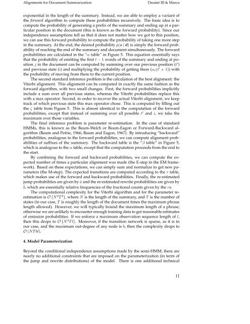
probabilities are calculated in the “α table” in Figure 5. This equation essentially says
that the probability of emitting the first t − 1 words of the summary and ending at position
j in the document can be computed by summing over our previous position (t ′ )
and previous state (i) and multiplying the probability of getting there (αi(t ′ + 1)) with
the probability of moving from there to the current position.
The second standard inference problem is the calculation of the best alignment: the
Viterbi alignment. This alignment can be computed in exactly the same fashion as the
forward algorithm, with two small changes. First, the forward probabilities implicitly
include a sum over all previous states, whereas the Viterbi probabilities replace this
with a max operator. Second, in order to recover the actual Viterbi alignment, we keep
track of which previous state this max operator chose. This is computed by filling out
the ζ table from Figure 5. This is almost identical to the computation of the forward
probabilities, except that instead of summing over all possible t ′ and i, we take the
maximum over those variables.
The final inference problem is parameter re-estimation. In the case of standard
HMMs, this is known as the Baum-Welch or Baum-Eagon or Forward-Backward algorithm
(Baum and Petrie, 1966; Baum and Eagon, 1967). By introducing “backward”
probabilities, analogous to the forward probabilities, we can compute alignment probabilities
of suffixes of the summary. The backward table is the “β table” in Figure 5,
which is analogous to the α table, except that the computation proceeds from the end to
the start.
By combining the forward and backward probabilities, we can compute the expected
number of times a particular alignment was made (the E-step in the EM framework).
Based on these expectations, we can simply sum and normalize to get new parameters
(the M-step). The expected transitions are computed according to the τ table,
which makes use of the forward and backward probabilities. Finally, the re-estimated
jump probabilities are given by â and the re-estimated rewrite probabilities are given by
ˆ b, which are essentially relative frequencies of the fractional counts given by the τs.
The computational complexity for the Viterbi algorithm and for the parameter reestimation
is O � N 2 T 2� , where N is the length of the summary, and T is the number of
states (in our case, T is roughly the length of the document times the maximum phrase
length allowed). However, we will typically bound the maximum length of a phrase;
otherwise we are unlikely to encounter enough training data to get reasonable estimates
of emission probabilities. If we enforce a maximum observation sequence length of l,
then this drops to O � N 2 T l � . Moreover, if the transition network is sparse, as it is in
our case, and the maximum out-degree of any node is b, then the complexity drops to
O (NT bl).
4. Model Parameterization
Beyond the conditional independence assumptions made by the semi-HMM, there are
nearly no additional constraints that are imposed on the parameterization (in term of
the jump and rewrite distributions) of the model. There is one additional technical
11