Peter Hamm and Martin T. Zanni - 2D IR spectroscopy

More documents

Recommendations

Info

2 we get zero as well. However, if we include the time propagation of such a density matrix: �� 1/2 −i/2e Tr(ρµ) = Tr iω01t +i/2e−iω01t � � 0 1 1/2 1 0 � −i/2eiωt 1/2 = Tr 1/2 i/2e−iωt � = sin ωt we see that it oscillates with amplitude one. Problem 2.3: Calculate the evolution of the density matrix for R2 and R5 in a manner that is analogous to Eq. 2.68. In what aspect are they different from R1 and R4? Solution: For R2 : � 1 0 0 0 and for R5 : � 1 0 0 0 � � iρµ0 0 i −→ � � +iω01t1 t1 0 ie −→ 0 0 0 0 � � � +iω01t1 ie 0 iµ2ρµ0µ1 0 0 −→ 0 0 ie +iω01t1 � t3 −→ 0 � 0 0 ie−iω01(t3−t1) � i〈µ3µ2ρµ0µ1〉 −→ ie 0 −iω01(t3−t1) � � iµ0ρ 0 0 −→ � −iω01t1 ie 0 � 0 0 0 0 ie−iω01(t3+t1) 0 i 0 � iµ2µ1µ0ρ −→ � � t1 −→ � 0 0 ie−iω01t1 0 � t3 −→ 0 0 ie −iω01t1 0 � i〈µ3µ2µ1µ0ρ〉 −→ ie −iω01(t3+t1) �� iρµ0µ1 −→ � iµ1µ0ρ −→ R2 and R5 have a ρ00 matrix element after the second field interaction, rather than a ρ11 matrix element. We say that these diagrams go through the ground state during the population time t2. Problem 2.4: Repeat the calculation of the propagation of the density matrix analogous to Eqns. 2.43, 2.44 and 2.50 with the first field interaction
acting from the left, however, now starting out from an excited state with: ρ(−∞) = � 0 0 0 1 Prove that E ∗ (t) ∝ e +iω01t now survives the rotating wave approximation, whereas the term related to E(t) ∝ e −iω01t vanishes. Draw the corresponding Feynman diagram. Solution: � 0 0 0 1 � iω01t1 ie 0 0 0 � � iµ0ρ 0 i −→ 0 0 � i〈µ0ρµ1〉 −→ ie iω01(t1) � . � � iω01t1 t1 0 ie −→ 0 0 � iµ0ρµ1 −→ Plugging this into Eq. 2.56, we get: P (1) (t) ∝ ie −iωt �∞ dt1E ′ (t − t1)e −t1/T2 +2iωt1 e 0 +ie +iωt � 0 ∞ dt1E ′ (t − t1)e −t1/T2 . (0.1) The term in the first integral is highly oscillating, hence the integral will be very small. 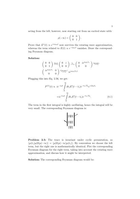The corresponding Feynman diagram is: 0 0 1 Problem 2.5: The trace is invariant under cyclic permutation, so 〈µ(t1)µ(0)ρ(−∞)〉 = 〈µ(0)ρ(−∞)µ(t1)〉. By convention we choose the left term, but the right one is mathematically identical. Plot the corresponding Feynman diagram for the right term, taking into account the rotating wave approximation, and discuss how it might be interpreted. Solution: The corresponding Feynman diagram would be: 0 1 1 3
Page 1: Concepts and Methods of 2D Infrared
Page 5: Problem 2.8: In Fig. 2.14, find the

Peter Hamm and Martin T. Zanni - 2D IR spectroscopy

You also want an ePaper? Increase the reach of your titles

Delete template?

Save as template?