S - UWSpace - University of Waterloo

More documents

Recommendations

Info

$uWaterloo LaTeX Thesis Template - UWSpace - University of Waterloo$

List of Symbols ∆ size of window in terms of time ɛ1, ɛ2 stopping rule thresholds UCL, LCL upper and lower control limit of control chart C κ distance of control limits from center line Λ weight matrix λ threshold for calculating frequent itemset candidates µ(S) mean value of S ν threshold for calculating the support of frequent itemsets ρ probability that a T 2 control chart has chi-square distribution σ(S) standard deviation of S τ significance level ω weight for calculating moving mean and standard deviation frequent itemset Ai A complete set of frequent itemsets in S AC cover set of A ASC smallest cover set of A Acc(Ri) the accuracy of the mining result Ri C control chart C candidate list for frequent itemsets mining d number of dimensions in multi-dimensional streams Gi partitions of a distribution gS i , gE i start and end point of partition Gi h bandwidth parameter for kernel density estimation H0 Null hypnosis that asserts distribution does not change Alternative hypnosis that asserts distribution has changed H1 xxi
Page 1 and 2: Mining Time-Changing Data Streams b
Page 3 and 4: Abstract Streaming data have gained
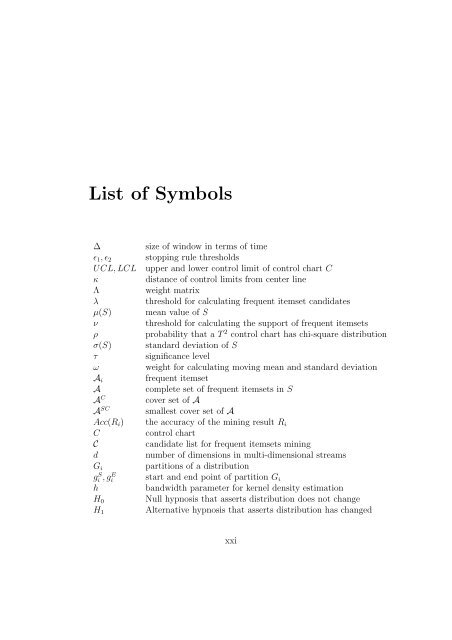
Page 5 and 6: Contents List of Figures ix List of
Page 7 and 8: 4 Change Detection in Multi-dimensi
Page 9 and 10: List of Figures 1.1 Abstract archit
Page 11 and 12: 3.30 Max duration for detecting tru
Page 13 and 14: 3.62 Max duration for detecting tru
Page 15 and 16: 3.96 Mean duration for detecting tr
Page 17 and 18: 3.129Number of true changes detecte
Page 19: List of Tables 3.1 Stream types gen
Page 23 and 24: Chapter 1 Introduction 1.1 Data str
Page 25 and 26: 4. Integrate stored and streaming D
Page 27 and 28: 1.1.4 Distribution changes in data
Page 29 and 30: the email sender/receiver locations
Page 31 and 32: changing data streams. These charac
Page 33 and 34: Unlike data mining algorithms that
Page 35 and 36: to be fine-tuned to improve perform
Page 37 and 38: a large amount of sample data to ac
Page 39: • A novel technique for mining fr
Page 42 and 43: 2.1 The data stream model 2.1.1 Dat
Page 44 and 45: Many window models have been propos
Page 46 and 47: S t t 1 t 2 Fixed window Landmark w
Page 48 and 49: over dynamic streams must find a
Page 50 and 51: and dropping more elements can spee
Page 52 and 53: Aggarwal et al. proposed a framewor
Page 54 and 55: pattern or a base time series with
Page 57 and 58: Chapter 3 Distribution Change Detec
Page 59 and 60: tures. Based on this insight, a con
Page 61 and 62: change occurs to the time it is det
Page 63 and 64: would greatly reduce the efficiency
Page 65 and 66: (a) (b) (c) S t 1 Timestamp last di
Page 67 and 68: 3.2, the accuracy of this estimatio
Page 69 and 70: substream S ′ r in the updated re
Page 71 and 72:
The location or scale (depends on t
Page 73 and 74:
to store the representative data se
Page 75 and 76:
changes mChg may not be the same as
Page 77 and 78:
stream speed is stable. However, no
Page 79 and 80:
Figure 3.4: Number of true changes
Page 81 and 82:
Figure 3.6: Number of false changes
Page 83 and 84:
Figure 3.8: Number of false changes
Page 85 and 86:
Figure 3.10: Mean duration for dete
Page 87 and 88:
Figure 3.12: Standard deviation of
Page 89 and 90:
Figure 3.14: Standard deviation of
Page 91 and 92:
0.000 0.005 0.010 0.015 0.020 0.025
Page 93 and 94:
The experimental results demonstrat
Page 95 and 96:
0.00 0.02 0.04 0.06 0.08 0.10 0.12
Page 97 and 98:
Figure 3.21: Number of false change
Page 99 and 100:
Figure 3.23: Number of false change
Page 101 and 102:
Figure 3.25: Mean duration for dete
Page 103 and 104:
0.00 0.05 0.10 0.15 Stream 8 − Un
Page 105 and 106:
0.000 0.005 0.010 0.015 Stream 12
Page 107 and 108:
0e+00 2e−04 4e−04 6e−04 8e−
Page 109 and 110:
The results of the second set of ex
Page 111 and 112:
0.00 0.02 0.04 0.06 0.08 0.10 0.12
Page 113 and 114:
0.00 0.05 0.10 0.15 0.00 0.02 0.04
Page 115 and 116:
0.00 0.02 0.04 0.06 0.08 0.00 0.05
Page 117 and 118:
0.000 0.002 0.004 0.006 0.008 0.010
Page 119 and 120:
0.000 0.005 0.010 0.015 0.020 0.000
Page 121 and 122:
0.00 0.02 0.04 0.06 0.000 0.002 0.0
Page 123 and 124:
0e+00 2e−04 4e−04 6e−04 8e−
Page 125 and 126:
0e+00 2e−04 4e−04 6e−04 0e+00
Page 127 and 128:
Since moving window method continuo
Page 129 and 130:
0.00 0.05 0.10 0.15 0.20 0.00 0.05
Page 131 and 132:
0.00 0.05 0.10 0.15 0.00 0.01 0.02
Page 133 and 134:
0.0 0.1 0.2 0.3 0.4 0.0 0.1 0.2 0.3
Page 135 and 136:
0.0 0.1 0.2 0.3 0.4 0.00 0.05 0.10
Page 137 and 138:
0.00 0.05 0.10 0.15 0.20 0.00 0.02
Page 139 and 140:
0.00 0.05 0.10 0.15 0.20 0.00 0.05
Page 141 and 142:
0.00 0.05 0.10 0.15 0.00 0.01 0.02
Page 143 and 144:
0.0 0.1 0.2 0.3 0.4 0.0 0.1 0.2 0.3
Page 145 and 146:
0.00 0.05 0.10 0.15 0.00 0.05 0.10
Page 147 and 148:
0.00 0.05 0.10 0.15 0.000 0.005 0.0
Page 149 and 150:
0.000 0.002 0.004 0.006 0.008 0.010
Page 151 and 152:
0.00 0.05 0.10 0.15 0.00 0.02 0.04
Page 153 and 154:
0.00 0.02 0.04 0.06 0.08 0.00 0.01
Page 155 and 156:
0.00 0.05 0.10 0.15 0.00 0.05 0.10
Page 157 and 158:
0.00 0.02 0.04 0.06 0.08 0.10 0.12
Page 159 and 160:
0.000 0.002 0.004 0.006 0.008 0.000
Page 161 and 162:
Note that in DMM the procedures of
Page 163 and 164:
Let Acc(Ri) be the accuracy of the
Page 165 and 166:
3.4 Detecting mean and standard dev
Page 167 and 168:
22 20 18 16 14 12 10 8 6 4 2 1 7 13
Page 169 and 170:
Significance level τ is the minimu
Page 171 and 172:
where τ is the significance level,
Page 173 and 174:
Algorithm 1 Mean and Standard Devia
Page 175 and 176:
0.00 0.02 0.04 0.06 0.08 0.10 0.12
Page 177 and 178:
0.00 0.05 0.10 0.15 Stream 5 − Mi
Page 179 and 180:
0.00 0.02 0.04 0.06 0.08 0.10 0.12
Page 181 and 182:
0.00 0.02 0.04 0.06 0.08 0.00 0.01
Page 183 and 184:
0.00 0.02 0.04 0.06 0.08 0.10 Strea
Page 185 and 186:
0.00 0.02 0.04 0.06 0.08 0.10 Contr
Page 187 and 188:
0.00 0.01 0.02 0.03 0.04 0.00 0.05
Page 189 and 190:
0.00 0.01 0.02 0.03 0.04 0.05 Strea
Page 191 and 192:
0.00 0.01 0.02 0.03 0.04 0.05 0.06
Page 193 and 194:
0.000 0.005 0.010 0.015 0.00 0.05 0
Page 195 and 196:
0.000 0.005 0.010 0.015 0.020 Strea
Page 197 and 198:
0.000 0.005 0.010 0.015 Control Cha
Page 199 and 200:
0.0000 0.0004 0.0008 0.0012 0.00 0.
Page 201 and 202:
0.0000 0.0005 0.0010 0.0015 Stream
Page 203 and 204:
0.0000 0.0005 0.0010 0.0015 Control
Page 205 and 206:
These results reveal that the propo
Page 207 and 208:
0.00 0.05 0.10 0.15 0.00 0.02 0.04
Page 209 and 210:
0.00 0.05 0.10 0.15 0.00 0.02 0.04
Page 211 and 212:
0.00 0.02 0.04 0.06 0.08 0.10 0.12
Page 213 and 214:
0.000 0.010 0.020 0.030 0.000 0.004
Page 215 and 216:
0.000 0.001 0.002 0.003 0.004 0.005
Page 217 and 218:
0.000 0.002 0.004 0.006 0.008 0.000
Page 219 and 220:
0.000 0.001 0.002 0.003 0.004 0e+00
Page 221 and 222:
Similar conclusions as the previous
Page 223 and 224:
0.00 0.01 0.02 0.03 0.04 0.05 0.06
Page 225 and 226:
0.00 0.05 0.10 0.15 0.000 0.001 0.0
Page 227 and 228:
These results suggest that, increas
Page 229 and 230:
0.00 0.02 0.04 0.06 0.08 0.00 0.02
Page 231 and 232:
0.000 0.010 0.020 0.030 0.000 0.004
Page 233:
3.5 Summary The unboundedness and h
Page 236 and 237:
to take more than one attribute int
Page 238 and 239:
probability distributions. However,
Page 240 and 241:
weight variables on each dimension
Page 242 and 243:
ta = t0. Null hypothesis H0 (i.e.,
Page 244 and 245:
element Xj = (x1, x2, ..., xd) ∈
Page 246 and 247:
into three sets. The first set cont
Page 248 and 249:
0.00 0.02 0.04 0.06 0.08 0.10 0.12
Page 250 and 251:
0.0 0.5 1.0 1.5 2.0 Num of False Ch
Page 252 and 253:
0.00 0.05 0.10 0.15 Num of True Cha
Page 254 and 255:
0.000 0.001 0.002 0.003 0.004 Max o
Page 256 and 257:
0.00 0.02 0.04 0.06 0.08 0.10 0.12
Page 258 and 259:
0.00 0.01 0.02 0.03 0.04 0.05 0.06
Page 261 and 262:
Chapter 5 Mining Frequent Itemsets
Page 263 and 264:
prediction window. All current freq
Page 265 and 266:
the problem of mining the complete
Page 267 and 268:
this approach cannot detect distrib
Page 269 and 270:
A time-based tumbling window WM, ca
Page 271 and 272:
• A counter for each itemset that
Page 273 and 274:
e discarded from the candidate list
Page 275 and 276:
Step 5.1. ∀Ak = {r} ∪ Ai, where
Page 277 and 278:
• Step 1. Let A SC = φ. Build a
Page 279 and 280:
Algorithm 4 MAINTAIN CANDIDATES 1:
Page 281 and 282:
transactions that are missed in cou
Page 283 and 284:
5.5 Experiments To evaluate TWIM’
Page 285 and 286:
as existing algorithms on streams w
Page 287 and 288:
Table 5.4: Mining results over S6 c
Page 289 and 290:
Varying window sizes To evaluate th
Page 291 and 292:
Table 5.11: Maximum counters when |
Page 293 and 294:
Chapter 6 Conclusions Many of today
Page 295 and 296:
ecause of these correlations. Very
Page 297:
itemsets, then a polynomial algorit
Page 300 and 301:
[9] F. Aparisi and J. Garcia-Diaz.
Page 302 and 303:
[29] J. Cheng, Y. Ke, and W. Ng. Ma
Page 304 and 305:
[49] W. Fan, Y. Huang, and P. Yu. D
Page 306 and 307:
[70] A. Hyvarinen. Survey on indepe
Page 308 and 309:
[92] A. Manjhi, S. Nath, and P. Gib
Page 310 and 311:
[113] M. Gertz et al. A data and qu
Page 312 and 313:
[134] M. Pelikan. Hierarchical baye
Page 314 and 315:
[156] A. Wald. Sequential Analysis.
show all

S - UWSpace - University of Waterloo

Create successful ePaper yourself

Delete template?

Save as template?