Solving DDEs in Matlab - Radford University

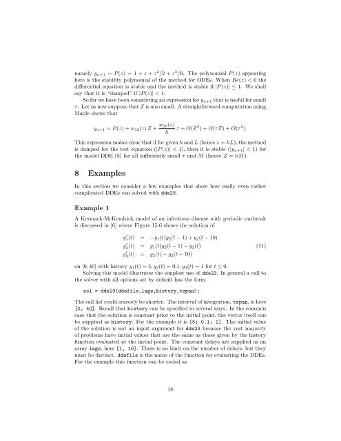
namely yn+1 = P (z) = 1 + z + z 2 /2 + z 3 /6. The polynomial P (z) appearing
here is the stability polynomial of the method for ODEs. When Re(z) < 0 the
differential equation is stable and the method is stable if |P (z)| ≤ 1. We shall
say that it is “damped” if |P (z)| < 1.
So far we have been considering an expression for yn+1 that is useful for small
τ. Let us now suppose that Z is also small. A straightforward computation using
Maple shows that
yn+1 = P (z) + w12(z) Z + w20(z)
h
τ + O(Z 2 ) + O(τZ) + O(τ 2 ).
This expression makes clear that if for given h and L (hence z = hL), the method
is damped for the test equation (|P (z)| < 1), then it is stable (|yn+1| < 1) for
the model DDE (8) for all sufficiently small τ and M (hence Z = hM).
8 Examples
In this section we consider a few examples that show how easily even rather
complicated DDEs can solved with dde23.
Example 1
A Kermack-McKendrick model of an infectious disease with periodic outbreak
is discussed in [6] where Figure 15.6 shows the solution of
y ′ 1(t) = −y1(t)y2(t − 1) + y2(t − 10)
y ′ 2(t) = y1(t)y2(t − 1) − y2(t) (11)
y ′ 3(t) = y2(t) − y2(t − 10)
on [0, 40] with history y1(t) = 5, y2(t) = 0.1, y3(t) = 1 for t ≤ 0.
Solving this model illustrates the simplest use of dde23. In general a call to
the solver with all options set by default has the form
sol = dde23(ddefile,lags,history,tspan);
The call list could scarcely be shorter. The interval of integration, tspan, is here
[0, 40]. Recall that history can be specified in several ways. In the common
case that the solution is constant prior to the initial point, the vector itself can
be supplied as history. For the example it is [5; 0.1; 1]. The initial value
of the solution is not an input argument for dde23 because the vast majority
of problems have initial values that are the same as those given by the history
function evaluated at the initial point. The constant delays are supplied as an
array lags, here [1, 10]. There is no limit on the number of delays, but they
must be distinct. ddefile is the name of the function for evaluating the DDEs.
For the example this function can be coded as
18