Stanford PNT hollberg Nov07 b - Stanford Center for Position ...
Stanford PNT hollberg Nov07 b - Stanford Center for Position ...
Stanford PNT hollberg Nov07 b - Stanford Center for Position ...

You also want an ePaper? Increase the reach of your titles
YUMPU automatically turns print PDFs into web optimized ePapers that Google loves.
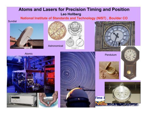
Sundial<br />
Atoms and Lasers <strong>for</strong> Precision Timing and <strong>Position</strong><br />
Leo Hollberg<br />
National Institute of Standards and Technology (NIST) , Boulder CO<br />
Atomic<br />
Astronomical<br />
Pendulum<br />
Harrison
Optical Frequency Measurements Group<br />
NIST, Boulder<br />
Optical Clocks<br />
Chris Oates<br />
Cold Ca<br />
Yann Le Coq → (SYRTE, Paris)<br />
Jason Stalnaker → (Oberlin)<br />
Guido Wilpers (Germany/NPL-UK)<br />
Anne Curtis (CU → NPL-UK)<br />
Kristin Beck (Rochester, SURF)<br />
Cold Yb<br />
Chad Hoyt (→ Bethel College)<br />
Zeb Barber (CU)<br />
Valeriey Yudin (Russia)<br />
Aleksei Taichanachev (Russia)<br />
Nathan Lemke (CU)<br />
Nicola Poli (LENS, Italy)<br />
Chip Scale Atomic Devices<br />
clocks, magnetometers …<br />
John Kitching<br />
Svenja Knappe (Germany)<br />
Peter Schwindt (Sandia)<br />
Vishal Shah → (Princeton)<br />
Vladi Gerginov (Bulgaria)<br />
Ying-Ju Wang (Taiwan)<br />
Clark Griffith<br />
Andy Geraci<br />
Hugh Robinson<br />
Liz Donley<br />
Eleanor Hodby (England)<br />
Alan Brannon (CU)<br />
Brad Lindseth (CU)<br />
Matt Eardley (CU)<br />
Susan Schima<br />
Lucas Willis (LSU, SURF)<br />
Nicolas VanMeter (SURF)<br />
•$$ NIST, DARPA-MTO, ONR-CU-MURI, NASA, LANL<br />
fs Frequency Combs<br />
Scott Diddams<br />
Tara Fortier (LANL)<br />
Jason Stalnaker → (Oberlin)<br />
Qudsia Quraishi (CU)<br />
Stephanie Meyer (C)U)<br />
Albrecht Bartels → (Konstance)<br />
L-S Ma, Z. Bi, (ECNU-BIPM)<br />
Y. Kobayashi (AIST Japan)<br />
Vela Mbele (South Africa)<br />
Matt Kirchner (CU)<br />
Andy Weiner* (Purdue)<br />
Danielle Braje<br />
Optical Length Metrology<br />
Richard Fox<br />
NIST Opto-Electronics<br />
Nate Newbury, Bill Swan ...
Accuracy of clocks through history<br />
Verge & Foliot Balance<br />
Year (AD)<br />
Primary Caesium Clocks<br />
Early Caesium Clocks<br />
Quartz Crystal<br />
Shortt<br />
Reifler<br />
Free Pendulum<br />
Harrison’s Chronometer<br />
Temperature Compensation<br />
Barometric Compensation<br />
Huygens Pendulum<br />
Chinese Hydro-mechanical<br />
Graham’s-Escapement<br />
Cross Beat Escapement<br />
1000 1200 1400 1600 1800 2000<br />
Future<br />
Fractional Error<br />
1ps / d<br />
1ns / d<br />
1 µs / d<br />
1ms / d<br />
1s / d<br />
1000 s / d<br />
Δt/t<br />
10 -15<br />
10 -9<br />
10 -3
Highest Accuracy Atomic Clocks
Current Microwave-Based Standards and Distribution<br />
Hydrogen<br />
Masers<br />
and<br />
Cesium<br />
Clocks<br />
NIST-F1<br />
NIST<br />
Measurement<br />
System<br />
Δf/f ~ 1x10 -15<br />
<strong>for</strong> standards<br />
and distribution<br />
Rb and/or Cs<br />
GPS<br />
Communications<br />
satellites<br />
Radio<br />
broadcasts<br />
Approaching the limit <strong>for</strong> standards and distribution systems.<br />
T. Parker et al.
Examples of Atomic Clocks <strong>for</strong> the Future Today ?<br />
• Optical Atomic clocks – use lasers rather than<br />
microwaves to probe atoms<br />
• CSAC (Chip Scale Atomic Clocks) <strong>for</strong> hand held portable<br />
systems<br />
Microwave Atomic frequency Standard<br />
Cs<br />
Microwave<br />
clock transition<br />
Laser cooling<br />
and detection<br />
852 nm<br />
9,192,163,707 Hz<br />
Laser Cooling<br />
and detection<br />
(Blue or UV)<br />
Optical Atomic frequency Standard<br />
Optical ‘Clock<br />
transition 10 15 Hz
Relative position, dimensional metrology, surveying instruments rely<br />
on the fixed speed of light c and frequency references<br />
discharge lamps, lasers and purely classical optics<br />
Michelson Interferometer,<br />
BIPM, Paris, circa 1910 ?<br />
HeNe 633 nm<br />
Frequency Lock<br />
electronics<br />
I 2<br />
Lunar ranging w/<br />
laser pulses<br />
" =<br />
c<br />
n!
NIST F1, Cs atomic fountain clock<br />
Primary frequency Std. of U.S.<br />
S. Jefferts, L. Donley, T. Heavner, T. Parker
Feedback System<br />
Locks LO to<br />
atomic resonance<br />
High-Q resonator<br />
Quartz<br />
Fabry Perot cavity<br />
Local Oscillator<br />
Generic Atomic Clock<br />
Microwave Synthesizer<br />
Laser<br />
Δν<br />
Atoms<br />
υ<br />
Counter<br />
Detector<br />
Ca<br />
456 986 240 494 158
Advantages of Optical Clocks Quantum Projection Noise<br />
Fractional Frequency instability ~<br />
1 P<br />
Cooling/<br />
detection<br />
transition<br />
S<br />
f<br />
3 P or D<br />
Clock<br />
transition<br />
0<br />
f optical<br />
microwave<br />
! = observation time<br />
N = number of atoms<br />
10<br />
!<br />
10<br />
0 !<br />
15<br />
10<br />
5<br />
10<br />
• Large number of atoms 10 6 or more<br />
• High signal/noise<br />
• Possibility of lattices<br />
# =<br />
One atomic clock is always “perfect”<br />
Two similar clocks -- hard to detect systematic errors<br />
Different types of clocks can determine most accurate and stable<br />
y<br />
K<br />
$ "<br />
"<br />
T<br />
N<br />
cycle<br />
atoms<br />
!<br />
Candidate neutral atoms<br />
Ca, Sr, Yb, Mg, H, Ag, Hg…<br />
0<br />
Δν<br />
ν 0<br />
ν
Laser source<br />
Ca Oven<br />
Optical Atomic Clocks<br />
Cold Atom Optical Frequency Reference<br />
I(f)<br />
0<br />
f r<br />
Optical Synthesizer<br />
Divider / Counter<br />
f n = nf r<br />
f<br />
µ-wave out<br />
optical out<br />
Stable optical<br />
Cavity
σ(τ)<br />
Oscillator Stability<br />
Ca<br />
Optical<br />
Cavities<br />
1 fs<br />
Cs<br />
Ca projected<br />
H-maser<br />
Hg +<br />
projected<br />
GPS<br />
1 day 1 month<br />
0.5 Hz @<br />
500 THZ
Fractional Frequency Uncertainty<br />
1.0E-09<br />
1.0E-10<br />
1.0E-11<br />
1.0E-12<br />
1.0E-13<br />
1.0E-14<br />
1.0E-15<br />
1.0E-16<br />
1.0E-17<br />
Accuracy of Atomic Frequency Standards - History<br />
state-of-the-art Cs microwave<br />
Infrared<br />
Visible<br />
Ion<br />
Alk. Earth<br />
1.0E-18<br />
1970 1975 1980 1985 1990<br />
Year<br />
1995 2000 2005 2010 2015
1 P1 (4s4p)<br />
423 nm cooling<br />
Δν = 34 MHz<br />
1 S0 (4s 2 ) m=0<br />
Percent of Atoms Excited<br />
40<br />
30<br />
20<br />
10<br />
Cold Calcium optical atomic clock<br />
3 P1 (4s4p) m=0<br />
657 nm clock<br />
Δν = 400 Hz<br />
0<br />
0 2 4 6 8 10 12<br />
Relative 657 nm Probe Detuning (MHz)<br />
5x10 6 atoms<br />
423 nm MOT<br />
Demodulated Signal (V)<br />
0.2<br />
0.1<br />
0.0<br />
-0.1<br />
-0.2<br />
Ca<br />
60 seconds data acquisition 400 Hz<br />
linewidth<br />
0 1000 2000 3000 4000<br />
Relative Probe Frequency (Hz)
1 P1 (6s6p)<br />
Atom number [a.u.]<br />
Ytterbium optical atomic clock<br />
- Excellent prospects <strong>for</strong> high stability and small absolute uncertainty<br />
398.9 nm,<br />
28 MHz<br />
3 P0 : 578.42 nm,<br />
~15 mHz<br />
Clock Transition<br />
full width ~ 4 Hz (Q >10 14 )<br />
0.55<br />
0.50<br />
0.45<br />
0.40<br />
0.35<br />
0.30<br />
0.25<br />
0.20<br />
0.15<br />
0.10<br />
0.05<br />
0.00<br />
-20 -15 -10 -5 0 5 10 15 20<br />
Frequency offset [Hz]<br />
Lattice<br />
759 nm<br />
3 P0,1,2 (6s6p)<br />
3 P1 : 555.8<br />
nm, 182 kHz<br />
Chad Hoyt<br />
Zeb Barber<br />
Chris Oates<br />
Candidates:<br />
Sr, Yb, Ca, Hg
Allan deviation σ y (τ)<br />
1E-14<br />
1E-15<br />
1E-16<br />
Stability of two optical freq. ref: Yb and Ca<br />
1 10 100<br />
Averaging time (s)<br />
1<br />
0.1<br />
Frequency precision [Hz]
Feedback System<br />
Locks LO to<br />
atomic resonance<br />
High-Q resonator<br />
Quartz<br />
Fabry Perot cavity<br />
Local Oscillator<br />
Generic Atomic Clock<br />
Microwave Synthesizer<br />
Laser<br />
Δν<br />
Atoms<br />
υ<br />
Counter<br />
Detector<br />
Ca<br />
456 986 240 494 158
Enthusiasm <strong>for</strong> Optical Atomic Clocks and fs Combs<br />
Tara<br />
Fortier<br />
Scott<br />
Diddams<br />
Nobel Prize<br />
2005<br />
Jan Hall<br />
Ted Hänsch
Count Optical Frequencies with Optical Frequency Combs<br />
Ultra-short and repetitive pulses of light<br />
20 fs<br />
time<br />
Ultrashort optical pulse, plus nonlinear fiber → Broad Spectum<br />
Repetitive pulse train → Frequency Comb → “ruler <strong>for</strong> frequency/time”<br />
Power<br />
Wavelength<br />
•Initial ef<strong>for</strong>ts/ideas: J. Eckstein, A. Ferguson & T. Hänsch (1978), V. P. Chebotayev (1988)
Self-Referenced Optical Frequency Sythesizer<br />
I(f)<br />
0<br />
Microwave out<br />
Jones, et al. Science 288, 635 (2000)<br />
Ideas, existed many places, Telle &<br />
Keller …, Udem, Hänsch …<br />
f n = n f rep + f o<br />
f o<br />
f rep<br />
x2 f 2n = 2nf rep + f o<br />
Pump<br />
f o<br />
532 nm<br />
convex<br />
Optical Freq. Ref<br />
f<br />
Ti:Sapphire<br />
Gain
The frequency of a mode is simply F N = N * f rep – f 0<br />
Where N is and integer ~ 10 6<br />
0<br />
f r =1/ τ r.t.<br />
f 0<br />
f rep ~ 1000 MHz<br />
0<br />
Frequency
500 THz<br />
Optical Oscillator<br />
CW Laser Output<br />
500 THz<br />
fs Pulse Train<br />
(Clock Output)<br />
Diddams, et al.<br />
~2 fs<br />
1 ns<br />
~5 x 10 5 Magnification<br />
time
Hg +<br />
~1 fs per<br />
tooth<br />
Mechanical Analogy of the Optical Clock<br />
Femtosecond Laser Comb<br />
1,000,000:1 Reduction Gear<br />
(not to scale)<br />
Microwave Output<br />
~1 ns per tooth<br />
Counter &<br />
Display
Applications of Optical Frequency Ref. and Combs<br />
•Advanced communication systems (security, autonomous synchronization)<br />
•Advanced Navigation (position determination and control)<br />
•Precise timing (moving into the fs range)<br />
•Tests of fundamental physics (special and general relativity, time variation of<br />
fundamental constants)<br />
•Sensors (strain, gravity, length metrology ……)<br />
•Ultrahigh speed data, multi-channel parallel broadcast, or receivers,<br />
coherent communications<br />
•Low noise microwaves, and electronic timing signals<br />
•Scientific applications ( precision spectroscopy, chemistry, trace gas<br />
detection… )<br />
•Quantum in<strong>for</strong>mation ( Ivan Deutsch …)<br />
•Fourier synthesized arbitrary wave<strong>for</strong>m generation
Optical<br />
reference<br />
f opt<br />
M3<br />
I(f)<br />
PUMP<br />
fs frequency combs as Optical Frequency Divider<br />
Generation of microwaves with low phase noise<br />
0<br />
f µ-wave<br />
M1 M2<br />
f<br />
Optical outputs<br />
µ-wave out<br />
OC<br />
20 fs<br />
I(f)<br />
f µ-wave = f opt /N<br />
time<br />
1 ns<br />
Microwave pulses<br />
30<br />
ps<br />
Microwave comb w/<br />
1 GHz mode spacing<br />
Microwave frequency<br />
f
L(f) dBc/Hz<br />
-40<br />
-60<br />
-80<br />
-100<br />
-120<br />
-140<br />
-160<br />
10 0<br />
Low phase-noise microwaves, 10 GHz<br />
atoms<br />
Cavity kT<br />
State of the art sapphire oscillator<br />
10 1<br />
10 2<br />
Optical Frequency<br />
Divider<br />
10 3<br />
Frequency (Hz)<br />
Opt. Divider Data from Hollberg et al. proceeds IEEE MWP meeting Oct. 04<br />
J. McFerran et al. Elect. Letter 2005<br />
Hg+ optical cavity<br />
State of the art microwave synthesizer<br />
10 4<br />
Photo detected shot-noise<br />
10 5<br />
10 6
Source Lab<br />
Laser Source<br />
563 nm<br />
linewidth ∆n
I(f)<br />
f rep<br />
GPS<br />
Optical Frequencies Measured via GPS<br />
optical<br />
x2<br />
Self-Referencing<br />
f unknown<br />
Fox et al. Applied Optics, 05,<br />
Even commercial systems now<br />
available – CLEO/QELS trade show<br />
f<br />
R. Fox, S. Diddams NIST,<br />
also similar work at NPL …<br />
Red, 633nm I 2 – Stabilized HeNe laser
Next generation Grace<br />
laser ranging ?<br />
Advanced cold atom clocks or<br />
Laser ranging/imaging in/from Space<br />
T2L2<br />
ESA<br />
PARCS<br />
NASA<br />
HYPER, …<br />
ACES<br />
ESA
NIST Time and Frequency<br />
John Kitching<br />
Svenja Knappe<br />
Vladislav Gerginov<br />
Vishal Shah<br />
CSAC<br />
Susan Schima<br />
Peter Schwindt<br />
Clark Griffith<br />
Brad Lindseth<br />
CSAM<br />
Ying-Ju Wang<br />
Matt Eardley<br />
Elizabeth Donley<br />
Eleanor Hodby<br />
Hugh G. Robinson<br />
NIST Electromagnetics<br />
John Moreland<br />
Li-Anne Liew<br />
Gyro<br />
CSADs Team<br />
Dir.<br />
Coup.<br />
MEMS<br />
University of Colorado<br />
Z. Popović<br />
A. Brannon LO<br />
J. Breitbarth<br />
J. Maclennan Wall coatings<br />
Y. Li
Chip Scale Atomic Devices<br />
CSAC (clock), CSAM (magnetometer), CSAG (gyro)<br />
Optical excitation, atoms, MEMS, VCSEL lasers, low power<br />
Battery powered devices, connect to application requirements
Cell Fabrication: Anodic Bonding<br />
• Pre<strong>for</strong>m created by KOH etching or<br />
DRIE of Si<br />
• Pyrex bonded on one side with<br />
anodic bonding<br />
• Cell pre<strong>for</strong>m filled with Cs<br />
– BaN 6 + CsCl → BaCl + Cs + 3N 2<br />
@ 150 ºC<br />
• Diced cells made at NIST using the<br />
anodic bonding technique<br />
– Interior: 1 mm x ∅ 0.9 mm<br />
– Exterior: 1.33 mm x (1.45 mm) 2<br />
L. Liew, et al., Appl. Phys. Lett., 84, 2694, 2004.<br />
1 mm<br />
1 mm<br />
Pyrex 7740 (125 µm)<br />
Silicon (375 µm)<br />
Pyrex 7740 (200 µm)
4.2 mm<br />
1.5 mm<br />
NIST Chip-Scale Atomic Clock: 2004<br />
1 mm<br />
S. Knappe, et al., Appl. Phys. Lett. 85, 1460 (2004).<br />
Volume:<br />
9.5 mm 3<br />
Cell volume:<br />
0.81 mm 3<br />
Cell temp:<br />
85 ºC<br />
Heating<br />
power:<br />
75 mW<br />
Stability:<br />
σ y (1 sec.) =<br />
2.5×10 -10
Short-term stability: 4×10 -11 @ 1 sec<br />
S. Knappe, et al., Opt. Express 13, 1249-<br />
1253 (2005).<br />
Relative Frequency<br />
(10 -9<br />
)<br />
4<br />
2<br />
0<br />
-2<br />
-4<br />
CSAC Frequency Stability<br />
1 mm<br />
20000 30000 40000 50000<br />
Time (sec)<br />
Longer-term stability: 1×10 -11 @ 1 hr<br />
S. Knappe, et al. Opt. Lett. 30, 2351-2353<br />
(2005).<br />
Allen Deviation, !f/f<br />
10 -9<br />
10 -10<br />
10 -11<br />
10 -12<br />
Drift<br />
Cs CSAC: -2 x 10 -8 /day<br />
87 Rb Cell:
(A Very Rough) Oscillator Comparison<br />
Adapted from figure by R. Lutwak, Symmetricom<br />
Quartz Crystal<br />
Oscillators
Applications of Microfabricated Atomic Clocks<br />
• Size (1 cm 3 )<br />
• Power (30 mW)<br />
Integration in portable,<br />
battery-operated devices<br />
• Precise timing: higher-per<strong>for</strong>mance, more reliable operation<br />
Key application areas:<br />
• Global positioning and navigation (GPS)<br />
• Faster acquisition time<br />
• More precise altitude determination<br />
• Direct P(Y)/M code acquisition → anti-jam capability<br />
• <strong>Position</strong> solution with < 4 satellites visible<br />
• Wireless communications, network synchronization<br />
• Fewer dropped cell phone calls<br />
• Avoidance of data accumulation<br />
• Data logging, seismology, remote sensors…<br />
• Others we don’t even know about
?<br />
GPS <strong>Position</strong>ing with < 4<br />
τ 3<br />
τ 4<br />
(τ 1 , τ 2 , τ 3 , τ 4 )<br />
(x, y, z, t)<br />
Satellites<br />
τ 2<br />
GPS<br />
Receiver<br />
Atomic<br />
clock<br />
τ 1
Commercialization of Chip-Scale Atomic Clocks<br />
Symmetricom/Draper/Sandia<br />
(courtesy R. Lutwak)<br />
RF output<br />
< 10 mW<br />
power requirement<br />
Complete functioning CSACs<br />
10 cm 3<br />
108 mW<br />
5×10 -11<br />
@ 100 s<br />
Honeywell<br />
(courtesy D. Youngner)<br />
solder<br />
titanium getter<br />
vcsel<br />
optical path<br />
optics<br />
vacuum<br />
Trans -Impedance Amp<br />
gold reflector<br />
rubidium +AR/N2<br />
solder<br />
Photo -detector<br />
top top cap cap<br />
wafer wafer<br />
cavity cavity cavity<br />
wafer wafer wafer<br />
bench bench bench bench wafer wafer wafer wafer<br />
1.7 cm 3<br />
57 mW<br />
4×10 -12<br />
@ 1 hr
Magnetometry with Chip-Scale Devices<br />
Atom Energy<br />
Hyperfine<br />
splitting<br />
-2 -1 0 +1 +2<br />
mFj ћω HF<br />
Zeeman splitting<br />
ћω L = ½µ ΒΒ
M X Magnetometer<br />
• Improved sensitivity; no GHz oscillator<br />
Energy<br />
D1<br />
Optical<br />
Microwave<br />
Vapor<br />
cell<br />
λ/4<br />
Filter<br />
A. Bloom, E. Alexandrov, A. Weis, and many others<br />
ν hf<br />
Photodetector<br />
B<br />
Semiconductor<br />
Laser<br />
ΔB<br />
RF<br />
Coils
Heater Currents<br />
Laser Current<br />
Local Oscillator<br />
Driving RF Coils<br />
Loop<br />
Filter<br />
Data<br />
Acquisition<br />
CSAM Operation<br />
Photo-<br />
Diode<br />
Signal<br />
Lock-in<br />
Amplifier<br />
2 kHz Sidebands<br />
Width = 1.7 kHz<br />
or 243 nT
M X CSAM Per<strong>for</strong>mance<br />
Sensitivity Frequency Response<br />
F 3dB = 1 kHz
Magnetocardiography with a CSAM<br />
• At U. Pittsburgh with Dr. V. Shusterman<br />
• Mouse anaesthetized, placed near CSAM<br />
• ECG and MCG signals recorded<br />
(a) (b)<br />
4.5 mm<br />
1<br />
2<br />
1.7 mm<br />
6<br />
5<br />
4<br />
3
CSAM Sensitivity Comparison<br />
Adapted from R. L. Fagaly,<br />
Rev. Sci. Instrum., 77 (2006).<br />
SQUID<br />
Susceptometry<br />
Geophysical<br />
Magnetocardiography Transient<br />
Electromagnetics<br />
Magnetic Anomaly<br />
Detection<br />
Non-Destructive Test and Evaluation<br />
2004<br />
Magnetoencephalography<br />
87 Rb, 1 mm 3 atom shot noise<br />
2006<br />
2005<br />
High Tc SQUID<br />
Low Tc SQUID
Nuclear Spin Gyroscopes<br />
• Much work in 1970s and 1980s<br />
– Fraser (1963), Bayley, Greenwood, Simpson (1973)<br />
– Commercial development: Litton, Singer-Kearfott, TI<br />
Alkali<br />
atom<br />
Spin<br />
Exchange<br />
129 Xe<br />
S (V)<br />
Noble gas<br />
atom<br />
Lock In signal<br />
Fit includes linear drift<br />
f=y0+c*x+a*exp(-x/d)*cos(2*3.14159265359*x/b)<br />
-0.2<br />
-0.3<br />
-0.4<br />
-0.5<br />
-0.6<br />
-0.7<br />
1e-1<br />
1e-2<br />
1e-3<br />
1e-4<br />
T 2 ~ 6 s<br />
-0.8<br />
0 5 10 15 20<br />
t (s)<br />
FFT of Lock-In Signal<br />
! = 100 us, S=200 mV<br />
Ω R<br />
M ng<br />
1<br />
B 0<br />
M Al<br />
N B0N<br />
R B !<br />
! + " 0<br />
ΔB 1 ΔB 2<br />
100 µs<br />
58 ms<br />
Time<br />
PD
OPTICS + atoms/molecules new capabilities<br />
• Cold atoms, stable lasers and femotosecond optical frequency combs<br />
having tremendous impact on fundamental science, precision measurements,<br />
and metrology<br />
• Optical/Laser era in frequency standards and precision timing, spectroscopy …<br />
• Already providing lowest phase-noise, timing jitter<br />
– fs jitter soon common place<br />
– Lowest phase noise microwave signals<br />
• Some applications of stable sources and combs<br />
– new capabilities <strong>for</strong> science fundamental physics<br />
– Ultralow timing jitter, ultrafast sampling A/D, synchronization<br />
– Frequency standard precision spanning the spectrum 1 GHz to 500 THz +<br />
– Stabilized fs optical frequency combs enabling several new directions in<br />
spectroscopy, Fourier synthesis<br />
• Chip Scale Atomic Devices – practical route to bring atomic precision to<br />
field devices<br />
– Combination of MEMS, diode lasers, atomic physics<br />
– Clocks, Magnetometers, Gyros ..