- Page 2 and 3:
BIOINFORMATICS ALGORITHMS
- Page 4 and 5:
Copyright © 2008 by John Wiley & S
- Page 6 and 7:
vi CONTENTS 6 A Survey of Seeding f
- Page 8 and 9:
PREFACE Bioinformatics, broadly def
- Page 10 and 11:
CONTRIBUTORS Sudha Balla, Departmen
- Page 12 and 13:
CONTRIBUTORS xiii Steven Hecht Orza
- Page 14 and 15:
1 EDUCATING BIOLOGISTS IN THE 21ST
- Page 16 and 17:
EDUCATING BIOLOGISTS IN THE 21ST CE
- Page 18 and 19:
EDUCATING BIOLOGISTS IN THE 21ST CE
- Page 20 and 21:
2 DYNAMIC PROGRAMMING ALGORITHMS FO
- Page 22 and 23:
SEQUENCE ALIGNMENT: GLOBAL, LOCAL,
- Page 24 and 25:
ecurrence: SEQUENCE ALIGNMENT: GLOB
- Page 26 and 27:
SEQUENCE ALIGNMENT: GLOBAL, LOCAL,
- Page 28 and 29:
SEQUENCE ALIGNMENT: GLOBAL, LOCAL,
- Page 30 and 31:
DYNAMIC PROGRAMMING ALGORITHMFOR RN
- Page 32 and 33:
DYNAMIC PROGRAMMING ALGORITHMFOR RN
- Page 34 and 35:
DYNAMIC PROGRAMMING ALGORITHMS FOR
- Page 36 and 37:
REFERENCES 25 the flexible structur
- Page 38 and 39:
REFERENCES 27 32. Gusfield D. Effic
- Page 40 and 41:
3 GRAPH THEORETICAL APPROACHES TO D
- Page 42 and 43:
GRAPH THEORY BACKGROUND 31 beginnin
- Page 44 and 45:
GRAPH THEORY BACKGROUND 33 FIGURE 3
- Page 46 and 47:
GRAPH THEORY BACKGROUND 35 chordal
- Page 48 and 49:
GRAPH THEORY BACKGROUND 37 decompos
- Page 50 and 51:
RECONSTRUCTING PHYLOGENIES 39 are (
- Page 52 and 53:
RECONSTRUCTING PHYLOGENIES 41 only
- Page 54 and 55:
FORMATION OF MULTIPROTEIN COMPLEXES
- Page 56 and 57:
3.4.1 Ribosomal Assembly FORMATION
- Page 58 and 59:
FORMATION OF MULTIPROTEIN COMPLEXES
- Page 60 and 61:
FORMATION OF MULTIPROTEIN COMPLEXES
- Page 62 and 63:
ACKNOWLEDGMENTS REFERENCES 51 This
- Page 64 and 65:
REFERENCES 53 37. Golumbic MC, Hart
- Page 66 and 67:
4 ADVANCES IN HIDDEN MARKOV MODELS
- Page 68 and 69:
HIDDEN MARKOV MODELS FOR SEQUENCE A
- Page 70 and 71:
HIDDEN MARKOV MODELS FOR SEQUENCE A
- Page 72 and 73:
HIDDEN MARKOV MODELS FOR SEQUENCE A
- Page 74 and 75:
ALTERNATIVES TO VITERBI DECODING 63
- Page 76 and 77:
Noncoding Coding Intron (a) Without
- Page 78 and 79:
also have this same label). We get
- Page 80 and 81:
change as follows: GENERALIZED HIDD
- Page 82 and 83:
0.00004 0.00002 0.00000 0 20000 400
- Page 84 and 85:
HMMS WITH MULTIPLE OUTPUTS OR EXTER
- Page 86 and 87:
HMMS WITH MULTIPLE OUTPUTS OR EXTER
- Page 88 and 89:
HMMS WITH MULTIPLE OUTPUTS OR EXTER
- Page 90 and 91:
HMMS WITH MULTIPLE OUTPUTS OR EXTER
- Page 92 and 93:
HMMS WITH MULTIPLE OUTPUTS OR EXTER
- Page 94 and 95:
TRAINING THE PARAMETERS OF AN HMM 8
- Page 96 and 97:
CONCLUSION 85 of parameters compare
- Page 98 and 99:
REFERENCES 87 4. Altun Y, Tsochanta
- Page 100 and 101:
REFERENCES 89 42. Krogh A. Using da
- Page 102 and 103:
REFERENCES 91 77. Xu EW, Kearney P,
- Page 104 and 105:
94 SORTING- AND FFT-BASED TECHNIQUE
- Page 106 and 107:
96 SORTING- AND FFT-BASED TECHNIQUE
- Page 108 and 109:
98 SORTING- AND FFT-BASED TECHNIQUE
- Page 110 and 111:
100 SORTING- AND FFT-BASED TECHNIQU
- Page 112 and 113:
102 SORTING- AND FFT-BASED TECHNIQU
- Page 114 and 115:
104 SORTING- AND FFT-BASED TECHNIQU
- Page 116 and 117:
106 SORTING- AND FFT-BASED TECHNIQU
- Page 118 and 119:
108 SORTING- AND FFT-BASED TECHNIQU
- Page 120 and 121:
110 SORTING- AND FFT-BASED TECHNIQU
- Page 122 and 123:
112 SORTING- AND FFT-BASED TECHNIQU
- Page 124 and 125:
114 SORTING- AND FFT-BASED TECHNIQU
- Page 126 and 127:
6 A SURVEY OF SEEDING FOR SEQUENCE
- Page 128 and 129:
ALIGNMENTS 119 6.2.1 Formal Definit
- Page 130 and 131:
TRADITIONAL APPROACHES TO HEURISTIC
- Page 132 and 133:
TRADITIONAL APPROACHES TO HEURISTIC
- Page 134 and 135:
TRADITIONAL APPROACHES TO HEURISTIC
- Page 136 and 137:
MORE CONTEMPORARY SEEDING APPROACHE
- Page 138 and 139:
MORE CONTEMPORARY SEEDING APPROACHE
- Page 140 and 141:
MORE CONTEMPORARY SEEDING APPROACHE
- Page 142 and 143:
MORE COMPLICATED SEED DESCRIPTIONS
- Page 144 and 145:
MORE COMPLICATED SEED DESCRIPTIONS
- Page 146 and 147:
MORE COMPLICATED SEED DESCRIPTIONS
- Page 148 and 149:
SOME THEORETICAL ISSUES IN ALIGNMEN
- Page 150 and 151:
REFERENCES 141 6. Brown DG. Optimiz
- Page 152 and 153:
7 THE COMPARISON OF PHYLOGENETIC NE
- Page 154 and 155:
INTRODUCTION 145 known phylogeny re
- Page 156 and 157:
BASIC DEFINITIONS 147 The undirecte
- Page 158 and 159:
BASIC DEFINITIONS 149 N1 displays N
- Page 160 and 161:
A B C A B C SUBTREES AND SUBNETWORK
- Page 162 and 163:
SUBTREES AND SUBNETWORKS 153 of x a
- Page 164 and 165:
SUBTREES AND SUBNETWORKS 155 1. it
- Page 166 and 167:
SUPERTREES AND SUPERNETWORKS 157 By
- Page 168 and 169:
SUPERTREES AND SUPERNETWORKS 159 Go
- Page 170 and 171:
SUPERTREES AND SUPERNETWORKS 161 Th
- Page 172 and 173:
RECONCILIATION OF GENE TREES AND SP
- Page 174 and 175:
RECONCILIATION OF GENE TREES AND SP
- Page 176 and 177:
RECONCILIATION OF GENE TREES AND SP
- Page 178 and 179:
RECONCILIATION OF GENE TREES AND SP
- Page 180 and 181:
RECONCILIATION OF GENE TREES AND SP
- Page 182 and 183:
REFERENCES 173 21. Gòrecki P, Tiur
- Page 184 and 185:
8 FORMAL MODELS OF GENE CLUSTERS An
- Page 186 and 187:
8.2 GENOME PLASTICITY 8.2.1 Genome
- Page 188 and 189:
GENOME PLASTICITY 181 FIGURE 8.2 An
- Page 190 and 191:
BASIC CONCEPTS 183 “more or less
- Page 192 and 193:
BASIC CONCEPTS 185 of {m, o, s}. On
- Page 194 and 195:
MODELS OF GENE CLUSTERS 187 Definit
- Page 196 and 197:
4, 2, 3, 1, 11, 10, 9, 8, 7, 6, 5 4
- Page 198 and 199:
MODELS OF GENE CLUSTERS 191 FIGURE
- Page 200 and 201:
MODELS OF GENE CLUSTERS 193 another
- Page 202 and 203:
MODELS OF GENE CLUSTERS 195 of gene
- Page 204 and 205:
MODELS OF GENE CLUSTERS 197 The two
- Page 206 and 207:
REFERENCES 199 flexibility by bound
- Page 208 and 209:
REFERENCES 201 28. Hoberman R, Dura
- Page 210 and 211:
9 INTEGER LINEAR PROGRAMMING TECHNI
- Page 212 and 213:
BASIC PROBLEM SPECIFICATION 205 a n
- Page 214 and 215:
INTEGER LINEAR PROGRAMMING FORMULAT
- Page 216 and 217:
INTEGER LINEAR PROGRAMMING FORMULAT
- Page 218 and 219:
9.4 EXTENSIONS AND VARIATIONS EXTEN
- Page 220 and 221:
i=1 EXTENSIONS AND VARIATIONS 213 H
- Page 222 and 223:
9.5 COMPUTATIONAL RESULTS COMPUTATI
- Page 224 and 225:
DISCUSSION 217 TABLE 9.2 Cluster Si
- Page 226 and 227:
DISCUSSION 219 FIGURE 9.5 Manually
- Page 228 and 229:
ACKNOWLEDGMENTS REFERENCES 221 We t
- Page 230 and 231:
224 EFFICIENT COMBINATORIAL ALGORIT
- Page 232 and 233:
226 EFFICIENT COMBINATORIAL ALGORIT
- Page 234 and 235:
228 EFFICIENT COMBINATORIAL ALGORIT
- Page 236 and 237:
230 EFFICIENT COMBINATORIAL ALGORIT
- Page 238 and 239:
232 EFFICIENT COMBINATORIAL ALGORIT
- Page 240 and 241:
234 EFFICIENT COMBINATORIAL ALGORIT
- Page 242 and 243:
236 EFFICIENT COMBINATORIAL ALGORIT
- Page 244 and 245:
238 EFFICIENT COMBINATORIAL ALGORIT
- Page 246 and 247:
11 ALGORITHMS FOR MULTIPLEX PCR PRI
- Page 248 and 249:
INTRODUCTION 243 problem: given a s
- Page 250 and 251:
1. p hybridizes at position t of f
- Page 252 and 253:
Thus, constraints 11.7 can be repla
- Page 254 and 255:
A GREEDY ALGORITHM 249 FIGURE 11.3
- Page 256 and 257:
EXPERIMENTAL RESULTS 251 11.5.1 Amp
- Page 258 and 259:
#primers/(2x#SNPs) (%) #primers/(2x
- Page 260 and 261:
TABLE 11.2 (Continued ) EXPERIMENTA
- Page 262 and 263:
REFERENCES 257 p, discard all candi
- Page 264 and 265:
12 RECENT DEVELOPMENTS IN ALIGNMENT
- Page 266 and 267:
12.2 MULTIPLE SEQUENCE ALIGNMENT 12
- Page 268 and 269:
MULTIPLE SEQUENCE ALIGNMENT 263 The
- Page 270 and 271:
MOTIF FINDING 265 Marsan and Sagot
- Page 272 and 273:
BIOLOGICAL NETWORK ANALYSIS 267 mul
- Page 274 and 275:
DISCUSSION 269 an interaction pair
- Page 276 and 277:
REFERENCES 271 13. Bucka-Lassen K,
- Page 278 and 279:
REFERENCES 273 52. Lee C, Grasso C,
- Page 280 and 281:
REFERENCES 275 90. Stormo GD, Hartz
- Page 282 and 283:
PART III MICROARRAY DESIGN AND DATA
- Page 284 and 285:
280 ALGORITHMS FOR OLIGONUCLEOTIDE
- Page 286 and 287:
282 ALGORITHMS FOR OLIGONUCLEOTIDE
- Page 288 and 289:
284 ALGORITHMS FOR OLIGONUCLEOTIDE
- Page 290 and 291:
286 ALGORITHMS FOR OLIGONUCLEOTIDE
- Page 292 and 293:
288 ALGORITHMS FOR OLIGONUCLEOTIDE
- Page 294 and 295:
290 ALGORITHMS FOR OLIGONUCLEOTIDE
- Page 296 and 297:
292 ALGORITHMS FOR OLIGONUCLEOTIDE
- Page 298 and 299:
294 ALGORITHMS FOR OLIGONUCLEOTIDE
- Page 300 and 301:
296 ALGORITHMS FOR OLIGONUCLEOTIDE
- Page 302 and 303:
298 ALGORITHMS FOR OLIGONUCLEOTIDE
- Page 304 and 305:
300 ALGORITHMS FOR OLIGONUCLEOTIDE
- Page 306 and 307:
14 CLASSIFICATION ACCURACY BASED MI
- Page 308 and 309:
INTRODUCTION 305 Decomposition (SVD
- Page 310 and 311:
METHODS 307 Note that in most of th
- Page 312 and 313: estimated as K� 1 ai,j = aik,j. d
- Page 314 and 315: METHODS 311 [7]. The KNN-classifier
- Page 316 and 317: ROWimpute-KNN ROWimpute-SVM KNNimpu
- Page 318 and 319: ROWimpute-KNN ROWimpute-SVM KNNimpu
- Page 320 and 321: Classification accuracies of SRBCT
- Page 322 and 323: ROWimpute-KNN ROWimpute-SVM KNNimpu
- Page 324 and 325: ROWimpute-KNN ROWimpute-SVM KNNimpu
- Page 326 and 327: Classification accuracies of SRBCT
- Page 328 and 329: REFERENCES 325 From these two plots
- Page 330 and 331: REFERENCES 327 18. Troyanskaya OG,
- Page 332 and 333: 330 META-ANALYSIS OF MICROARRAY DAT
- Page 334 and 335: 332 META-ANALYSIS OF MICROARRAY DAT
- Page 336 and 337: 334 META-ANALYSIS OF MICROARRAY DAT
- Page 338 and 339: 336 META-ANALYSIS OF MICROARRAY DAT
- Page 340 and 341: 338 META-ANALYSIS OF MICROARRAY DAT
- Page 342 and 343: 340 META-ANALYSIS OF MICROARRAY DAT
- Page 344 and 345: 342 META-ANALYSIS OF MICROARRAY DAT
- Page 346 and 347: 344 META-ANALYSIS OF MICROARRAY DAT
- Page 348 and 349: 346 META-ANALYSIS OF MICROARRAY DAT
- Page 350 and 351: 348 META-ANALYSIS OF MICROARRAY DAT
- Page 352 and 353: 350 META-ANALYSIS OF MICROARRAY DAT
- Page 354 and 355: 352 META-ANALYSIS OF MICROARRAY DAT
- Page 356 and 357: 16 PHASING GENOTYPES USING A HIDDEN
- Page 358 and 359: A HIDDEN MARKOV MODEL FOR RECOMBINA
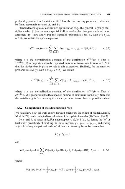
- Page 360 and 361: LEARNING THE HMM FROM UNPHASED GENO
- Page 364 and 365: LEARNING THE HMM FROM UNPHASED GENO
- Page 366 and 367: EXPERIMENTAL RESULTS 365 It is also
- Page 368 and 369: DISCUSSION 367 TABLE 16.1 Phasing A
- Page 370 and 371: GERBIL PHASE fastPHASE 0.4 0.35 0.3
- Page 372 and 373: REFERENCES 371 however, that direct
- Page 374 and 375: 17 ANALYTICAL AND ALGORITHMIC METHO
- Page 376 and 377: INTRODUCTION 375 The use of real ha
- Page 378 and 379: follows: X11 = 2N11 + N12 + N21 X21
- Page 380 and 381: METHODS 379 FIGURE 17.1 The likelih
- Page 382 and 383: METHODS 381 TABLE 17.3 Tests for Ha
- Page 384 and 385: METHODS 383 The sixth stochastic al
- Page 386 and 387: RESULTS 385 TABLE 17.4 The Distribu
- Page 388 and 389: RESULTS 387 TABLE 17.6 The Distribu
- Page 390 and 391: DISCUSSION 389 2SNP also produced r
- Page 392 and 393: ACKNOWLEDGMENTS 391 haplotypes need
- Page 394 and 395: REFERENCES 393 16. Hill WG. Estimat
- Page 396 and 397: 18 OPTIMIZATION METHODS FOR GENOTYP
- Page 398 and 399: Tag-restricted haplotype n Complete
- Page 400 and 401: INFORMATIVE SNP SELECTION 399 from
- Page 402 and 403: DISEASE ASSOCIATION SEARCH 401 18.2
- Page 404 and 405: DISEASE ASSOCIATION SEARCH 403 18.3
- Page 406 and 407: Below is the formal description of
- Page 408 and 409: RESULTS AND DISCUSSION 407 to decid
- Page 410 and 411: RESULTS AND DISCUSSION 409 � Comp
- Page 412 and 413:
RESULTS AND DISCUSSION 411 TABLE 18
- Page 414 and 415:
RESULTS AND DISCUSSION 413 nonindex
- Page 416 and 417:
REFERENCES 415 20. Lee PH, Shatkay
- Page 418 and 419:
19 TOPOLOGICAL INDICES IN COMBINATO
- Page 420 and 421:
TOPOLOGICAL INDICES 421 The quantit
- Page 422 and 423:
Theorem 19.2 Let T = (V, E) be a tr
- Page 424 and 425:
HOSOYA POLYNOMIAL 425 The Laplacian
- Page 426 and 427:
H2(G, x) = � {u,v}⊆V INVERSE WI
- Page 428 and 429:
HEXAGONAL SYSTEMS 429 hexagonal sys
- Page 430 and 431:
C 2 HEXAGONAL SYSTEMS 431 FIGURE 19
- Page 432 and 433:
THE WIENER INDEX OF PEPTOIDS 433 Th
- Page 434 and 435:
if R ≥ L, then π(Lp) = i; Lp = L
- Page 436 and 437:
REFERENCES 437 19. Entringer RC, Me
- Page 438 and 439:
20 EFFICIENT ALGORITHMS FOR STRUCTU
- Page 440 and 441:
COMPOUND REPRESENTATION 441 FIGURE
- Page 442 and 443:
COMPOUND REPRESENTATION 443 breakag
- Page 444 and 445:
TABLE 20.1 Bond List of Aspirin Bon
- Page 446 and 447:
COMPOUND REPRESENTATION 447 20.2.5
- Page 448 and 449:
Initial class value for node A A 3
- Page 450 and 451:
CHEMICAL COMPOUND DATABASE 451 In c
- Page 452 and 453:
CHEMICAL COMPOUND DATABASE 453 taki
- Page 454 and 455:
CHEMICAL COMPOUND DATABASE 455 Othe
- Page 456 and 457:
REFERENCES 457 lab may take months
- Page 458 and 459:
REFERENCES 459 22. Curco D, Rodrigu
- Page 460 and 461:
REFERENCES 461 61. An J, Nakama T,
- Page 462 and 463:
REFERENCES 463 101. Shen J. HAD An
- Page 464 and 465:
466 COMPUTATIONAL APPROACHES TO PRE
- Page 466 and 467:
468 COMPUTATIONAL APPROACHES TO PRE
- Page 468 and 469:
470 COMPUTATIONAL APPROACHES TO PRE
- Page 470 and 471:
472 COMPUTATIONAL APPROACHES TO PRE
- Page 472 and 473:
474 COMPUTATIONAL APPROACHES TO PRE
- Page 474 and 475:
476 COMPUTATIONAL APPROACHES TO PRE
- Page 476 and 477:
478 COMPUTATIONAL APPROACHES TO PRE
- Page 478 and 479:
480 COMPUTATIONAL APPROACHES TO PRE
- Page 480 and 481:
482 COMPUTATIONAL APPROACHES TO PRE
- Page 482 and 483:
484 COMPUTATIONAL APPROACHES TO PRE
- Page 484 and 485:
486 COMPUTATIONAL APPROACHES TO PRE
- Page 486 and 487:
488 COMPUTATIONAL APPROACHES TO PRE
- Page 488 and 489:
490 COMPUTATIONAL APPROACHES TO PRE
- Page 490 and 491:
INDEX 2SNP computer program 383, 38
- Page 492 and 493:
degeneracy 101-104, 112 degenerate
- Page 494 and 495:
lowest p-value method 484-486 max-g
- Page 496 and 497:
pseudoknots 20 p-value 339-343, 347
- Page 498:
ioinformatics-cp.qxd 11/29/2007 8:4