ejercicio de calculo de incertidumbre aplicado a la ley de ohm
ejercicio de calculo de incertidumbre aplicado a la ley de ohm
ejercicio de calculo de incertidumbre aplicado a la ley de ohm

Create successful ePaper yourself
Turn your PDF publications into a flip-book with our unique Google optimized e-Paper software.
EJERCICIO DE CALCULO DE INCERTIDUMBRE<br />
APLICADO A LA LEY DE OHM<br />
O. Gutiérrez<br />
CENAM, Laboratorio Multifunciones<br />
km 4,5 Carretera a los Cués El Marqués Qro<br />
Tel. 01 42 11 05 00, Fax 01 42 11 15 38, ogutierr@cenam.mx<br />
Resumen: En los <strong>la</strong>boratorios <strong>de</strong> calibración <strong>de</strong>l área eléctrica <strong>de</strong>l país comúnmente se realizan mediciones<br />
indirectas con base en <strong>la</strong> Ley <strong>de</strong> Ohm, aunque su cálculo <strong>de</strong> <strong>incertidumbre</strong> asociado es re<strong>la</strong>tivamente sencillo,<br />
representa un número significativo <strong>de</strong> horas hombre, el método presentado en este documento preten<strong>de</strong> hacer<br />
más eficiente esta tarea, pero sobre todo, busca promover que dicho cálculo se realimente al proceso <strong>de</strong><br />
medición.<br />
INTRODUCCION<br />
Cuando se lee el resumen <strong>de</strong>l método para <strong>la</strong><br />
evaluación y expresión <strong>de</strong> <strong>la</strong> <strong>incertidumbre</strong> que<br />
propone <strong>la</strong> Guía BIMP [1] se encuentra que el primer<br />
paso es expresar matemáticamente <strong>la</strong> re<strong>la</strong>ción entre<br />
el mensurando y los argumentos, tratándose <strong>de</strong> una<br />
medición indirecta con base en <strong>la</strong> Ley <strong>de</strong> Ohm resulta<br />
c<strong>la</strong>ra <strong>la</strong> formalización ya que normalmente no están<br />
involucradas magnitu<strong>de</strong>s <strong>de</strong> influencia y <strong>la</strong>s<br />
magnitu<strong>de</strong>s <strong>de</strong> <strong>de</strong>finición están re<strong>la</strong>cionadas por<br />
operaciones básicas (suma, resta, división o<br />
multiplicación). En estos casos se presentan dos<br />
alternativas para realizar el cálculo <strong>de</strong> <strong>incertidumbre</strong>:<br />
<strong>la</strong> primera es manejar <strong>la</strong>s componentes y resultados<br />
<strong>de</strong> manera absoluta, en otras pa<strong>la</strong>bras en <strong>la</strong>s<br />
unida<strong>de</strong>s <strong>de</strong> que se trate (A, Ω ó V) o <strong>la</strong> segunda en<br />
forma re<strong>la</strong>tiva al valor <strong>de</strong> interés (%, ppm,<br />
mUnida<strong>de</strong>s/Unida<strong>de</strong>s o μUnida<strong>de</strong>s/Unida<strong>de</strong>s).<br />
Ambas alternativas conducen a los mismos<br />
resultados, sin embargo el manejar <strong>la</strong>s componentes<br />
en forma absoluta (A, Ω ó V) triplica el tiempo<br />
invertido en respecto al involucrado cuando se tratan<br />
<strong>de</strong> forma re<strong>la</strong>tiva, esta diferencia se agudiza a<br />
medida que se involucran mas elementos como son:<br />
aplicación <strong>de</strong> los certificados <strong>de</strong> calibración,<br />
correcciones por estabilidad, linealidad o potencia<br />
disipada.<br />
Cuando se maneja gran<strong>de</strong>s conjuntos <strong>de</strong> datos como<br />
en <strong>la</strong> calibración <strong>de</strong> un equipo multifunción, resulta<br />
crítico <strong>la</strong> manipu<strong>la</strong>ción <strong>de</strong> <strong>la</strong> información, por en<strong>de</strong> es<br />
muy recomendable trabajar con mo<strong>de</strong>los sintetizados<br />
y manejar cantida<strong>de</strong>s re<strong>la</strong>tivas respecto a valores<br />
nominales en vez <strong>de</strong> lecturas directas. Este <strong>ejercicio</strong><br />
está orientado <strong>de</strong> esta forma y es el resumen <strong>de</strong> <strong>la</strong><br />
experiencia <strong>de</strong> calibrar calibradores y multímetros <strong>de</strong><br />
alta exactitud.<br />
DESARROLLO<br />
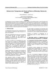
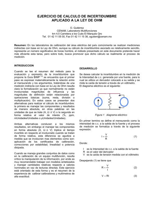
Se <strong>de</strong>sea calcu<strong>la</strong>r <strong>la</strong> <strong>incertidumbre</strong> en <strong>la</strong> medición <strong>de</strong><br />
<strong>la</strong> Intensidad <strong>de</strong> c.c. generada por una fuente, para lo<br />
cual se utiliza un <strong>de</strong>rivador colocado a su salida y se<br />
mi<strong>de</strong> <strong>la</strong> caída <strong>de</strong> tensión a través <strong>de</strong> un vóltmetro.<br />
El diagrama eléctrico es el siguiente:<br />
Figura 1 diagrama eléctrico<br />
En primer termino se <strong>de</strong>fine el mensurando como <strong>la</strong><br />
intensidad <strong>de</strong> c.c. a <strong>la</strong> salida <strong>de</strong> <strong>la</strong> fuente y el proceso<br />
<strong>de</strong> medición se formaliza a través <strong>de</strong> <strong>la</strong> siguiente<br />
expresión:<br />
Don<strong>de</strong>:<br />
V<br />
I = (1)<br />
R<br />
I es <strong>la</strong> Intensidad <strong>de</strong> c.c. a <strong>la</strong> salida <strong>de</strong> <strong>la</strong> fuente<br />
R es el valor <strong>de</strong>l <strong>de</strong>rivador<br />
V es <strong>la</strong> caída <strong>de</strong> tensión medida con el vóltmetro<br />
Despejando (1) se tiene que<br />
v<br />
V<br />
R = (2)<br />
I<br />
V = RI<br />
(3)
A continuación se calcu<strong>la</strong>n los coeficientes <strong>de</strong><br />
sensibilidad <strong>de</strong>rivando (1) en función <strong>de</strong> sus<br />
componentes y se simplifican a través <strong>de</strong> (2) y (3).<br />
∂I<br />
1<br />
= =<br />
∂V<br />
R<br />
∂I<br />
V<br />
= −<br />
∂R<br />
R<br />
2<br />
1<br />
V<br />
I<br />
=<br />
I<br />
V<br />
RI I<br />
= − = − 2<br />
R R<br />
Se asumen Funciones <strong>de</strong> Distribución <strong>de</strong><br />
Probabilidad (FDP) para cada una <strong>de</strong> <strong>la</strong>s<br />
componentes con base en <strong>la</strong> información disponible y<br />
se <strong>de</strong>termina una FDP resultante <strong>de</strong> su convolución,<br />
<strong>la</strong> cuál será asociada al mensurando.<br />
Usualmente en estos procesos <strong>de</strong> convolución se<br />
satisface el teorema <strong>de</strong> límite central que establece<br />
que: “La distribución <strong>de</strong> probabilidad <strong>de</strong>l mensurando<br />
Y será aproximadamente Normal si <strong>la</strong>s magnitu<strong>de</strong>s<br />
<strong>de</strong> <strong>de</strong>finición Xi <strong>de</strong>l mensurando son in<strong>de</strong>pendientes<br />
entre sí, y si <strong>la</strong> varianza <strong>de</strong>l mensurando σ 2 (Y) es<br />
mucho mayor que <strong>la</strong> varianza <strong>de</strong> cualquier magnitud<br />
<strong>de</strong> <strong>de</strong>finición σ 2 (Xi) que no sea Normal” [1] .<br />
La <strong>incertidumbre</strong> estándar combinada está dada por<br />
<strong>la</strong> siguiente expresión:<br />
u<br />
u<br />
2<br />
c<br />
2<br />
c<br />
⎛ ∂I<br />
⎞<br />
⎜ ⎟<br />
⎝ ∂V<br />
⎠<br />
2<br />
2<br />
( I)<br />
= u ( V)<br />
+ u ( R)<br />
⎛ I ⎞<br />
⎜ ⎟<br />
⎝ V ⎠<br />
2<br />
2<br />
⎛<br />
⎜<br />
⎝<br />
⎛ ∂I<br />
⎞<br />
⎜ ⎟<br />
⎝ ∂R<br />
⎠<br />
I ⎞<br />
⎟<br />
R ⎠<br />
2<br />
2<br />
( I)<br />
= u ( V)<br />
+ − u ( R)<br />
Manipu<strong>la</strong>ndo <strong>la</strong> expresión anterior queda como:<br />
u<br />
2<br />
c<br />
u<br />
2<br />
2<br />
( I)<br />
= * u ( V)<br />
+ * u ( R)<br />
2<br />
c<br />
2<br />
I<br />
⎛ uc<br />
⎜<br />
⎝ I<br />
I<br />
V<br />
2<br />
2<br />
2<br />
2<br />
( I)<br />
u ( V)<br />
u ( R)<br />
=<br />
V<br />
2<br />
* +<br />
( ) ( ) ( ) 2<br />
2<br />
2<br />
I u V u R<br />
⎞<br />
⎟<br />
⎠<br />
⎛<br />
= ⎜<br />
⎝<br />
V<br />
⎞<br />
⎟<br />
⎠<br />
R<br />
I<br />
R<br />
2<br />
2<br />
2<br />
⎛<br />
+ ⎜<br />
⎝ R<br />
2<br />
2<br />
⎞<br />
⎟<br />
⎠<br />
Multiplicando ambos miembros <strong>de</strong> <strong>la</strong> igualdad por<br />
(10 6 ) 2 se tiene:<br />
⎛ u<br />
⎜<br />
⎝<br />
c<br />
2<br />
6<br />
6<br />
2<br />
( I)<br />
* 10 ⎞ ⎛ u(<br />
V)<br />
* 10 ⎞ ⎛ u(<br />
R)<br />
I<br />
⎟<br />
⎠<br />
=<br />
⎜<br />
⎝<br />
V<br />
⎟<br />
⎠<br />
+<br />
⎜⎜<br />
⎝<br />
* 10<br />
R<br />
6<br />
2<br />
⎞<br />
⎟⎟<br />
⎠<br />
Las <strong>incertidumbre</strong>s quedan expresadas en forma<br />
re<strong>la</strong>tiva a <strong>la</strong> lectura y por lo tanto pue<strong>de</strong> escribirse<br />
como:<br />
u<br />
2<br />
c Ω<br />
2<br />
2<br />
( μA /A )( I)<br />
= u μV/V<br />
( V)<br />
+ u μΩ/<br />
( R)<br />
(4)<br />
Se observa en <strong>la</strong> expresión anterior que el manejo <strong>de</strong><br />
<strong>la</strong>s componentes <strong>de</strong> <strong>incertidumbre</strong> en forma re<strong>la</strong>tiva<br />
implica que los coeficientes <strong>de</strong> sensibilidad sean<br />
unitarios y por tanto ambas magnitu<strong>de</strong>s tengan <strong>la</strong><br />
misma pon<strong>de</strong>ración. La expresión (4) pue<strong>de</strong><br />
acomodarse para Tensión y Resistencia Eléctrica y<br />
es igualmente válida.<br />
u<br />
u<br />
2<br />
c A<br />
2<br />
2<br />
( μ Ω/<br />
Ω)(<br />
R)<br />
= uμV<br />
/ V ( V)<br />
+ uμA<br />
/ ( I)<br />
2<br />
c I Ω<br />
2<br />
2<br />
( μV/V )( V)<br />
= uμA<br />
/ A(<br />
) + uμΩ/<br />
( R)<br />
Ahora en el contexto <strong>de</strong> una calibración el<br />
mensurando es el error re<strong>la</strong>tivo <strong>de</strong> <strong>la</strong> fuente y <strong>la</strong><br />
formalización está dada por:<br />
Don<strong>de</strong>:<br />
⎛ L − I⎞<br />
6<br />
E = ⎜ ⎟ * 10<br />
(5)<br />
⎝ I ⎠<br />
L es el valor seleccionado en <strong>la</strong> fuente.<br />
I es el valor medido a través <strong>de</strong> <strong>de</strong>rivador y el<br />
vóltmetro, el cual se calcu<strong>la</strong> con base en <strong>la</strong><br />
expresión (1)<br />
Con <strong>la</strong> finalidad <strong>de</strong> facilitar <strong>la</strong> aplicación <strong>de</strong> los<br />
informes <strong>de</strong> calibración, <strong>la</strong>s correcciones por<br />
estabilidad, linealidad y potencia disipada se<br />
manipu<strong>la</strong> <strong>la</strong> expresión (5) para poner<strong>la</strong> en términos<br />
<strong>de</strong> valores re<strong>la</strong>tivos partiendo <strong>de</strong> <strong>la</strong>s tres<br />
consi<strong>de</strong>raciones siguientes:<br />
a) La lectura <strong>de</strong>l vóltmetro “Vsimple” se corrige a partir<br />
<strong>de</strong> su informe <strong>de</strong> calibración aplicando <strong>la</strong><br />
siguiente expresión general:<br />
V<br />
corregida<br />
Vsimple<br />
= (6)<br />
( 1+<br />
E′<br />
)<br />
<strong>la</strong> cual proviene <strong>de</strong> <strong>la</strong> fórmu<strong>la</strong> <strong>de</strong>l error re<strong>la</strong>tivo y<br />
don<strong>de</strong>, para facilitar el <strong>de</strong>sarrollo, se utiliza <strong>la</strong><br />
siguiente notación:<br />
EV<br />
E ′ V =<br />
(7)<br />
6<br />
10<br />
El valor EV es el error re<strong>la</strong>tivo <strong>de</strong>l vóltmetro<br />
reportado en su informe <strong>de</strong> calibración.<br />
V
) La lectura <strong>de</strong>l vóltmetro pue<strong>de</strong> expresarse en<br />
términos re<strong>la</strong>tivos como:<br />
⎡med − nom ⎤ 6<br />
= * 10 (8)<br />
V V<br />
Ä V ⎢<br />
⎥<br />
⎣ nom V ⎦<br />
Don<strong>de</strong> nomV es <strong>la</strong> caída <strong>de</strong> tensión nominal que<br />
se espera en el <strong>de</strong>rivador y medV es <strong>la</strong> indicación<br />
<strong>de</strong>l vóltmetro Entonces <strong>de</strong>spejando medV en (8)<br />
se tiene:<br />
V<br />
( 1 Ä′<br />
V ) med V<br />
nom * + =<br />
(9)<br />
c) Por último el valor <strong>de</strong> resistencia eléctrica <strong>de</strong> un<br />
<strong>de</strong>rivador <strong>de</strong> corriente pue<strong>de</strong> expresarse en<br />
términos re<strong>la</strong>tivos como:<br />
Ä<br />
R<br />
⎡nomR − R⎤<br />
6<br />
= ⎢<br />
* 10<br />
⎣ R ⎥<br />
(10)<br />
⎦<br />
Don<strong>de</strong> nomR es el valor nominal <strong>de</strong> resistencia<br />
eléctrica <strong>de</strong>l <strong>de</strong>rivador <strong>de</strong> corriente y “R” es su<br />
valor real. Entonces <strong>de</strong>spejando “R” en (10) se<br />
tiene:<br />
nomR<br />
R = (11)<br />
1+<br />
Ä′<br />
Sustituyendo (6), (9) y (11) en (1):<br />
V<br />
I = =<br />
R<br />
med<br />
V<br />
( 1+<br />
E′<br />
)<br />
nom<br />
V<br />
R<br />
( 1+<br />
Ä′<br />
)<br />
R<br />
=<br />
Desarrol<strong>la</strong>ndo se tiene:<br />
I<br />
I<br />
⎡nom<br />
⎤<br />
*<br />
V<br />
= ⎢ ⎥<br />
⎣nomR<br />
⎦<br />
⎡nom<br />
⎤<br />
*<br />
V<br />
= ⎢ ⎥<br />
⎣nomR<br />
⎦<br />
Sí se cumple que:<br />
nom<br />
R<br />
V * ( 1+<br />
Ä′<br />
V )<br />
( 1+<br />
E′<br />
)<br />
nom<br />
V<br />
R<br />
( 1+<br />
Ä′<br />
)<br />
R<br />
( 1+<br />
Ä′<br />
V )( 1+<br />
ÄR′<br />
)<br />
( 1+<br />
E′<br />
)<br />
V<br />
( 1+<br />
Ä′<br />
V + ÄR′<br />
+ Ä′<br />
V ÄR′<br />
)<br />
( 1+<br />
E′<br />
)<br />
nom V<br />
= nomI<br />
y Ä ′ V ÄR′<br />
〈〈 Ä′<br />
V ≈ Ä′<br />
R<br />
nomR<br />
Entonces (12) queda como:<br />
V<br />
(12)<br />
I = nom<br />
I<br />
*<br />
( 1+<br />
Ä′<br />
V + ÄR′<br />
)<br />
( 1+<br />
E′<br />
)<br />
V<br />
Multiplicando ambos miembros <strong>de</strong> <strong>la</strong> igualdad por 1<br />
resulta que:<br />
I = nom<br />
I = nom<br />
Como:<br />
( E ) 1<br />
2<br />
〈〈<br />
V<br />
I<br />
I<br />
*<br />
*<br />
( 1+<br />
Ä′<br />
V + Ä′<br />
R)<br />
( 1+<br />
E′<br />
)<br />
V<br />
*<br />
( 1−<br />
E′<br />
V )<br />
( 1−<br />
E′<br />
)<br />
( 1+<br />
Ä′<br />
V + ÄR′<br />
− E′<br />
V − Ä′<br />
VE′<br />
V − ÄR′<br />
E′<br />
V )<br />
2<br />
1−<br />
( E′<br />
)<br />
V<br />
( V )<br />
′ y Ä ′ V ≈ ÄR′<br />
≈ E′<br />
V 〉〉 Ä′<br />
VE′<br />
V ≈ ÄR′<br />
E′<br />
V<br />
Entonces se tiene que:<br />
I<br />
( 1 + Ä′<br />
+ Ä′<br />
− E )<br />
I = nom *<br />
′<br />
(13)<br />
Sustituyendo (13) en (5)<br />
V<br />
R<br />
* ( 1+<br />
Ä′<br />
V + ÄR′<br />
− E′<br />
V )<br />
( 1+<br />
Ä′<br />
+ Ä′<br />
− E′<br />
)<br />
⎛ L − nom<br />
⎞ 6<br />
= * 10 (14)<br />
⎝<br />
⎠<br />
I<br />
EI nomI<br />
*<br />
⎟<br />
V R V<br />
⎟<br />
⎜<br />
“L” es <strong>la</strong> selección en <strong>la</strong> fuente y por lo tanto es igual<br />
al valor nominal <strong>de</strong> Intensidad <strong>de</strong> c.c. “nomI,“ a<strong>de</strong>más<br />
en el <strong>de</strong>nominador se pue<strong>de</strong> hacer <strong>la</strong> siguiente<br />
simplificación:<br />
nom * 1+<br />
Ä′<br />
+ Ä′<br />
− E′<br />
= nom<br />
Entonces (14) queda como:<br />
E<br />
I<br />
I<br />
V<br />
( V R V ) I<br />
( L − nom ) − nom * ( Ä′<br />
+ Ä′<br />
− E ) ⎞ 6<br />
⎛ ′<br />
I I V R<br />
=<br />
⎜<br />
⎝<br />
nomI<br />
Simplificando se tiene que:<br />
I<br />
6<br />
( Ä′<br />
+ Ä′<br />
− E ) * 10<br />
E = −<br />
′<br />
V<br />
R<br />
Con base en <strong>la</strong> expresión (7) queda como:<br />
I<br />
V<br />
( Ä + Ä E )<br />
V<br />
R<br />
V<br />
V<br />
⎟ * 10<br />
⎠<br />
E = − −<br />
(15)<br />
La aplicación <strong>de</strong> <strong>la</strong> expresión (15) reduce al cálculo a<br />
una suma <strong>de</strong> cantida<strong>de</strong>s sencil<strong>la</strong>s en partes por<br />
millón “ppm” o porcentajes:<br />
E I<br />
=<br />
−<br />
( 5,2ppm<br />
+ 4,1ppm<br />
− 2,1ppm)<br />
= −7,2ppm
Hasta este punto solo se ha manipu<strong>la</strong>do <strong>la</strong><br />
formalización <strong>de</strong>l proceso <strong>de</strong> medición, ahora se<br />
calcu<strong>la</strong>rán los coeficientes <strong>de</strong> sensibilidad <strong>de</strong>rivando<br />
el mensurando “EI” respecto a cada componente.<br />
∂E<br />
∂Δ<br />
I =<br />
V<br />
-1<br />
∂E<br />
∂Δ<br />
I =<br />
R<br />
-1<br />
∂E<br />
∂E<br />
I<br />
V<br />
= 1<br />
Paso seguido se calcu<strong>la</strong> <strong>la</strong> <strong>incertidumbre</strong> estándar<br />
combina con base en <strong>la</strong> siguiente expresión:<br />
2<br />
⎛ ∂E<br />
⎞<br />
⎜ ⎟<br />
I 2<br />
I 2<br />
I 2<br />
( E ) = u ( Ä ) + u ( Ä ) + u ( E )<br />
uc I<br />
V<br />
R ⎟<br />
⎝ ∂Δ<br />
V ⎠ ⎝ ∂ΔR<br />
⎠ ⎝ ∂EV<br />
⎠<br />
c<br />
2<br />
⎛ ∂E<br />
⎞<br />
⎜ ⎟<br />
2<br />
⎛ ∂E<br />
⎞<br />
⎜<br />
2 2<br />
2 2<br />
2 2<br />
( E ) = ( - 1)<br />
u ( Ä ) + ( - 1)<br />
u ( Ä ) ( 1)<br />
u ( E )<br />
u +<br />
c<br />
I<br />
V<br />
2<br />
2<br />
2<br />
( E ) u ( Ä ) + u ( Ä ) u ( E )<br />
u = +<br />
(16)<br />
I<br />
V<br />
R<br />
A continuación <strong>de</strong> estima <strong>la</strong> <strong>incertidumbre</strong> estándar<br />
<strong>de</strong> cada una <strong>de</strong> <strong>la</strong>s componentes:<br />
a) Para u 2 (ΔV) se tiene:<br />
rsl<br />
s<br />
2<br />
V(<br />
ppm ⎜ ) V ⎟ ⎜ ( ppm)<br />
u =<br />
(17)<br />
( Ä )<br />
V<br />
⎛<br />
⎜<br />
⎝<br />
2<br />
3<br />
⎞<br />
⎟<br />
⎠<br />
2<br />
⎛<br />
+<br />
⎜<br />
⎝<br />
R<br />
V<br />
n<br />
2<br />
⎟ ⎟<br />
⎞<br />
⎠<br />
La primer parte correspon<strong>de</strong> a <strong>la</strong> resolución <strong>de</strong>l<br />
Vóltmetro y es tratada como una Función <strong>de</strong><br />
Distribución <strong>de</strong> Probabilidad (FDP) rectangu<strong>la</strong>r, <strong>la</strong><br />
segunda es <strong>de</strong>bida a <strong>la</strong> variabilidad <strong>de</strong> <strong>la</strong>s<br />
lecturas <strong>de</strong>l mismo instrumento y es evaluada<br />
como tipo “A” don<strong>de</strong> “n” es el número <strong>de</strong><br />
mediciones, ambas expresadas en forma re<strong>la</strong>tiva.<br />
b) Para u 2 (ρ) se tiene:<br />
2<br />
⎛ ⎞<br />
2 ⎛ ucal(R)<br />
⎞ ⎛ uest(R)<br />
⎞ upot<br />
(R)<br />
u ( Ä )<br />
+ + ⎜ ⎟<br />
R = ⎜<br />
⎟<br />
⎜<br />
⎟<br />
⎜ ⎟<br />
⎝ k cal ⎠ ⎝ k est ⎠ ⎝ k pot ⎠<br />
2<br />
V<br />
V<br />
2<br />
(18)<br />
La primer parte correspon<strong>de</strong> a <strong>la</strong> <strong>incertidumbre</strong><br />
<strong>de</strong> calibración <strong>de</strong>l <strong>de</strong>rivador, <strong>la</strong> siguiente a su<br />
estabilidad y <strong>la</strong> última es <strong>de</strong>bida a <strong>la</strong> diferencia <strong>de</strong><br />
<strong>la</strong> intensidad <strong>de</strong> prueba con <strong>la</strong> que fue calibrado<br />
respecto a <strong>la</strong> que se <strong>de</strong>sea medir en el momento<br />
<strong>de</strong> uso. Los <strong>de</strong>nominadores <strong>de</strong>notados con <strong>la</strong><br />
letra “k” correspon<strong>de</strong>n al factor <strong>de</strong> cobertura al<br />
que están reportados cada una <strong>de</strong> <strong>la</strong>s<br />
componentes.<br />
c) Para u 2 (EV) se tiene:<br />
2<br />
2 ⎛ u ⎛ ⎞ ⎛ ⎞<br />
cal(E<br />
V ) ⎞ u est(E<br />
V ) u lin(E<br />
V )<br />
u ( EV<br />
) =<br />
⎜<br />
⎟ +<br />
⎜<br />
⎟ +<br />
⎜<br />
⎟<br />
⎝ k cal ⎠ ⎝ k est ⎠ ⎝ k lin ⎠<br />
2<br />
2<br />
(19)<br />
La primer parte correspon<strong>de</strong> a <strong>la</strong> <strong>incertidumbre</strong><br />
<strong>de</strong> calibración <strong>de</strong>l Vóltmetro, <strong>la</strong> siguiente a su<br />
estabilidad y <strong>la</strong> última es <strong>de</strong>bida a <strong>la</strong> linealidad si<br />
es que <strong>la</strong> caída <strong>de</strong> tensión medida con el<br />
Vóltmetro al momento <strong>de</strong> uso es diferente al<br />
punto en que fue calibrado.<br />
Sustituyendo expresiones (17), (18) y (19) en (16)<br />
⎛ rsl<br />
2<br />
V<br />
u ( E ) =<br />
⎜<br />
I<br />
⎜ 2<br />
⎝<br />
s<br />
( ppm)<br />
V(<br />
ppm)<br />
3<br />
⎛ ucal(R)<br />
⎞<br />
+ ⎜<br />
⎟<br />
⎝ k cal ⎠<br />
⎞<br />
⎟<br />
⎟<br />
⎠<br />
2<br />
2<br />
2<br />
⎛<br />
+<br />
⎜<br />
⎜<br />
⎝<br />
2<br />
⎞<br />
⎟<br />
⎟<br />
⎠<br />
⎛ u ⎛ ⎞<br />
est(R)<br />
⎞ upot<br />
(R)<br />
+ + ⎜ ⎟<br />
⎜<br />
⎟<br />
⎜ ⎟<br />
⎝ k est ⎠ ⎝ k pot ⎠<br />
⎛ u ⎞ ⎛ ⎞ ⎛<br />
cal(EV<br />
) uest(EV<br />
) ulin(E<br />
+<br />
⎜<br />
⎟ +<br />
⎜<br />
⎟ +<br />
⎜<br />
⎝ k cal ⎠ ⎝ k est ⎠ ⎝ klin<br />
2<br />
2<br />
2<br />
V<br />
) ⎞<br />
⎟<br />
⎠<br />
A continuación se presenta un <strong>ejercicio</strong> práctico<br />
don<strong>de</strong> se mi<strong>de</strong> una fuente que genera <strong>de</strong>s<strong>de</strong> 1 a 10 A<br />
y se asignan valores para cada una <strong>de</strong> <strong>la</strong>s<br />
componentes i<strong>de</strong>ntificadas en <strong>la</strong> expresión anterior.<br />
Intensidad <strong>de</strong><br />
c.c. (A)<br />
ursl(ΔV)<br />
ppm<br />
utipoA(ΔV)<br />
ppm<br />
ucal(ΔR)<br />
ppm<br />
uest(ΔR)<br />
ppm<br />
n<br />
upot(ΔR)<br />
μΩ/Ω ppm<br />
ucal(EV)<br />
ppm<br />
uest(EV)<br />
ppm<br />
ulin(EV)<br />
ppm<br />
c<strong>la</strong>ve 1 2 3 4 5 6 7 8<br />
2<br />
uc(I)<br />
ppm<br />
1 1.0 0.5 2.0 5.0 5.9 1.0 1.5 15 17.1<br />
2 0.5 0.3 2.0 5.0 5.8 1.0 1.5 7.5 11.0<br />
3 0.3 0.2 2.0 5.0 5.5 1.0 1.5 5.0 9.3<br />
4 0.3 0.1 2.0 5.0 5.0 1.0 1.5 3.8 8.5<br />
5 0.2 0.1 2.0 5.0 4.5 1.0 1.5 3.0 7.8<br />
6 0.2 0.1 2.0 5.0 3.8 1.0 1.5 2.5 7.3<br />
7 0.1 0.1 2.0 5.0 3.1 1.0 1.5 2.1 6.8<br />
8 0.1 0.1 2.0 5.0 2.2 1.0 1.5 1.9 6.4<br />
9 0.1 0.1 2.0 5.0 1.1 1.0 1.5 1.7 6.0<br />
10 0.1 0.1 2.0 5.0 0.0 1.0 1.5 1.5 5.9<br />
Tab<strong>la</strong> 1 componentes <strong>de</strong> <strong>incertidumbre</strong> iniciales<br />
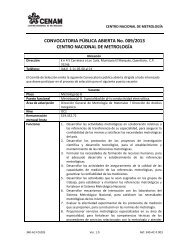
Para cada una <strong>de</strong> <strong>la</strong>s componentes se asigna una<br />
c<strong>la</strong>ve con <strong>la</strong> que se i<strong>de</strong>ntifican en <strong>la</strong> gráfica siguiente:
18.0<br />
16.0<br />
14.0<br />
12.0<br />
10.0<br />
8.0<br />
6.0<br />
4.0<br />
2.0<br />
0.0<br />
8<br />
17.1<br />
11.0<br />
9.3<br />
8<br />
7.8<br />
7.3<br />
6.8<br />
6.4<br />
5<br />
5<br />
5<br />
6.0 5.9<br />
4 4 84<br />
45 4<br />
5<br />
4 4 4 4 4<br />
8<br />
8.5<br />
8<br />
5<br />
8<br />
3<br />
7<br />
61 3<br />
7<br />
6<br />
3<br />
7<br />
6<br />
3<br />
7<br />
6<br />
3<br />
7<br />
6<br />
3<br />
7<br />
6<br />
8<br />
3<br />
7<br />
6<br />
83<br />
5<br />
7<br />
6<br />
3<br />
78 65 3<br />
78<br />
6<br />
2 1<br />
2 1<br />
2 12 12 12 12 12 12 51<br />
2<br />
1.0 2.0 3.0 4.0 5.0 6.0 7.0 8.0 9.0 10.0<br />
Intensidad <strong>de</strong> c.c. (A)<br />
Gráfica 1 componentes <strong>de</strong> <strong>incertidumbre</strong> iniciales<br />
De <strong>la</strong> gráfica se pue<strong>de</strong> observar que para valores<br />
bajos <strong>de</strong> intensidad <strong>de</strong> corriente <strong>la</strong> componente<br />
principal es <strong>de</strong>bida a <strong>la</strong> linealidad <strong>de</strong>l vóltmetro (c<strong>la</strong>ve<br />
8) y para valores altos es <strong>la</strong> <strong>de</strong>bida a <strong>la</strong> estabilidad<br />
<strong>de</strong>l <strong>de</strong>rivador (c<strong>la</strong>ve 4). Entonces resulta dos<br />
acciones <strong>de</strong> mejora al sistema <strong>de</strong> medición, en primer<br />
término se calibrará el vóltmetro en <strong>la</strong> parte baja <strong>de</strong>l<br />
intervalo para disminuir <strong>la</strong> componente por linealidad,<br />
<strong>la</strong> segunda acción es poner bajo seguimiento<br />
metrológico al <strong>de</strong>rivador para disminuir <strong>la</strong><br />
<strong>incertidumbre</strong> por estabilidad, aplicando ambas<br />
correcciones los nuevos valores <strong>de</strong> <strong>la</strong> tab<strong>la</strong> serían:<br />
Intensidad <strong>de</strong><br />
c.c. (A)<br />
ursl(ΔV)<br />
ppm<br />
utipoA(ΔV)<br />
ppm<br />
ucal(ΔR)<br />
ppm<br />
uest(ΔR)<br />
ppm<br />
upot(ΔR)<br />
μΩ/Ω ppm<br />
5<br />
ucal(EV)<br />
ppm<br />
uest(EV)<br />
ppm<br />
ulin(EV)<br />
ppm<br />
c<strong>la</strong>ve 1 2 3 4 5 6 7 8<br />
uc(I)<br />
ppm<br />
1 1.0 0.5 2.0 2.5 5.9 1.0 1.5 1.5 7.2<br />
2 0.5 0.3 2.0 2.5 5.8 1.0 1.5 1.5 7.0<br />
3 0.3 0.2 2.0 2.5 5.5 1.0 1.5 1.5 6.8<br />
4 0.3 0.1 2.0 2.5 5.0 1.0 1.5 1.5 6.4<br />
5 0.2 0.1 2.0 2.5 4.5 1.0 1.5 1.5 6.0<br />
6 0.2 0.1 2.0 2.5 3.8 1.0 1.5 1.5 5.5<br />
7 0.1 0.1 2.0 2.5 3.1 1.0 1.5 1.5 5.0<br />
8 0.1 0.1 2.0 2.5 2.2 1.0 1.5 1.5 4.5<br />
9 0.1 0.1 2.0 2.5 1.1 1.0 1.5 1.5 4.1<br />
10 0.1 0.1 2.0 2.5 0.0 1.0 1.5 1.5 4.0<br />
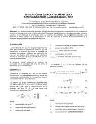
Tab<strong>la</strong> 2 componentes <strong>de</strong> <strong>incertidumbre</strong> finales<br />
La gráfica entonces queda como se muestra a<br />
continuación.<br />
8.0<br />
7.0<br />
6.0<br />
5.0<br />
4.0<br />
3.0<br />
2.0<br />
1.0<br />
0.0<br />
5<br />
5<br />
5<br />
5<br />
5<br />
4 4 4 4 4 4 4 4 4 4<br />
5<br />
3 3 3 3 3 3 3 3 3 3<br />
78 78 78 78 78 78 78 78 78 78<br />
5<br />
61 6 6 6 6 6 6 6 6 6<br />
2<br />
7.2<br />
1<br />
2<br />
7.0<br />
6.8<br />
6.4<br />
6.0<br />
5<br />
5.5<br />
1<br />
2<br />
1<br />
2<br />
1<br />
2 1<br />
2 12 12 12 1<br />
52<br />
1.0 2.0 3.0 4.0 5.0 6.0 7.0 8.0 9.0 10.0<br />
Intensidad <strong>de</strong> c.c. (A)<br />
Gráfica 2 componentes <strong>de</strong> <strong>incertidumbre</strong> finales<br />
En esta gráfica se observa <strong>la</strong> “penalización” en<br />
<strong>incertidumbre</strong> que se paga por utilizar el <strong>de</strong>rivador a<br />
una intensidad diferente a <strong>la</strong> que fue calibrado.<br />
Es pertinente mencionar que <strong>de</strong>be existir una razón<br />
c<strong>la</strong>ra porque reducir <strong>la</strong> <strong>incertidumbre</strong>, dicha razón<br />
<strong>de</strong>be ser fundada en <strong>la</strong>s necesida<strong>de</strong>s <strong>de</strong> un proceso<br />
o sistema y no solo motivada por <strong>la</strong> búsqueda <strong>de</strong>l<br />
conocimiento por sí mismo. El mejor sistema <strong>de</strong><br />
medición es aquel que satisface <strong>la</strong> necesidad <strong>de</strong><br />
manera eficiente y no siempre es el <strong>de</strong> menor<br />
<strong>incertidumbre</strong> asociada.<br />
La <strong>incertidumbre</strong> no es el enemigo a vencer sino <strong>la</strong><br />
brúju<strong>la</strong> <strong>de</strong>l metrólogo que lo orienta en su tarea<br />
diaria.<br />
CONCLUSIONES<br />
El expresar <strong>la</strong>s componentes <strong>de</strong> <strong>incertidumbre</strong> en<br />
forma re<strong>la</strong>tiva a <strong>la</strong> lectura facilita <strong>la</strong> estimación <strong>de</strong><br />
<strong>incertidumbre</strong> y su realimentación al proceso <strong>de</strong><br />
medición.<br />
REFERENCIAS<br />
[1] Guía BIPM/ISO Para <strong>la</strong> Expresión <strong>de</strong> <strong>la</strong><br />
Incertidumbre en <strong>la</strong>s Mediciones, 1990.<br />
5<br />
5.0<br />
4.5<br />
4.1<br />
4.0