la incertidumbre expandida y los grados de libertad - Centro ...
la incertidumbre expandida y los grados de libertad - Centro ...
la incertidumbre expandida y los grados de libertad - Centro ...

Create successful ePaper yourself
Turn your PDF publications into a flip-book with our unique Google optimized e-Paper software.
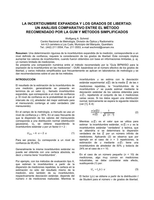
LA INCERTIDUMBRE EXPANDIDA Y LOS GRADOS DE LIBERTAD:<br />
UN ANÁLISIS COMPARATIVO ENTRE EL MÉTODO<br />
RECOMENDADO POR LA GUM Y MÉTODOS SIMPLIFICADOS<br />
Wolfgang A. Schmid<br />
<strong>Centro</strong> Nacional <strong>de</strong> Metrología, División <strong>de</strong> Óptica y Radiometría<br />
km 4,5 carretera a Los Cués, Municipio <strong>de</strong>l Marqués, Querétaro<br />
Tel.: (442) 211 0554, Fax: 211 0553, e-mail wschmid@cenam.mx<br />
Resumen: Una <strong>de</strong>terminación rigurosa <strong>de</strong> <strong>la</strong> <strong>incertidumbre</strong> <strong>expandida</strong> <strong>de</strong> <strong>la</strong> medición, correspondiente a un<br />
nivel <strong>de</strong>finido <strong>de</strong> confianza, requiere <strong>la</strong> consi<strong>de</strong>ración <strong>de</strong> <strong>los</strong> <strong>grados</strong> <strong>de</strong> <strong>libertad</strong>. Este concepto implica<br />
aumentar <strong>los</strong> valores <strong>de</strong> <strong>incertidumbre</strong>, cuando fueron obtenidos con base en informaciones limitadas, p. ej.<br />
un número limitado <strong>de</strong> mediciones.<br />
Se presenta una comparación numérica entre el método recomendado por <strong>la</strong> “Guía BIPM/ISO para <strong>la</strong><br />
expresión <strong>de</strong> <strong>la</strong> <strong>incertidumbre</strong> en <strong>la</strong>s mediciones“ - GUM, basándose en el número efectivo <strong>de</strong> <strong>los</strong> <strong>grados</strong> <strong>de</strong><br />
<strong>libertad</strong>, y varios métodos simplificados que frecuentemente se aplican en <strong>la</strong>boratorios <strong>de</strong> metrología y se<br />
dan recomendaciones sobre el uso <strong>de</strong> <strong>los</strong> métodos.<br />
INTRODUCCIÓN<br />
El resultado <strong>de</strong> <strong>la</strong> estimación <strong>de</strong> <strong>la</strong> <strong>incertidumbre</strong> <strong>de</strong><br />
una medición, generalmente se presenta en<br />
terminos <strong>de</strong> un valor Up , l<strong>la</strong>mado <strong>incertidumbre</strong><br />
<strong>expandida</strong>, que correspon<strong>de</strong> a un nivel <strong>de</strong> confianza<br />
p. El nivel <strong>de</strong> confianza es <strong>la</strong> probabilidad <strong>de</strong> que el<br />
intervalo <strong>de</strong> ±Up alre<strong>de</strong>dor <strong>de</strong>l mejor estimado para<br />
el mensurando contenga al valor verda<strong>de</strong>ro (<strong>de</strong>l<br />
mensurando).<br />
En el campo <strong>de</strong> <strong>la</strong> metrología, a menudo se usa un<br />
nivel <strong>de</strong> confianza p ≅ 95%. En el caso frecuente <strong>de</strong><br />
que <strong>la</strong> dispersión <strong>de</strong> <strong>los</strong> valores <strong>de</strong>l mensurando<br />
corresponda a una distribución normal (distribución<br />
gaussiana), Up se obtiene expandiendo <strong>la</strong><br />
<strong>incertidumbre</strong> estándar u por un factor k = 2 :<br />
U = k ⋅u<br />
= 2 ⋅u<br />
95 %<br />
(1)<br />
Para ser preciso, 2u correspon<strong>de</strong> a un nivel <strong>de</strong><br />
confianza <strong>de</strong> 95,45%.<br />
Generalmente <strong>la</strong> misma <strong>incertidumbre</strong> estándar no<br />
pue<strong>de</strong> ser obtenida con una certeza absoluta, es<br />
<strong>de</strong>cir u misma tiene “<strong>incertidumbre</strong>“.<br />
Por ejemplo, con <strong>los</strong> métodos <strong>de</strong> evaluación tipo A,<br />
que estiman <strong>la</strong> <strong>incertidumbre</strong> a partir <strong>de</strong> <strong>la</strong><br />
dispersión <strong>de</strong> mediciones repetidas, <strong>la</strong> certeza en <strong>la</strong><br />
estimación no sólo <strong>de</strong>l resultado mismo <strong>de</strong> <strong>la</strong><br />
medición, sino también <strong>de</strong> su <strong>incertidumbre</strong>,<br />
respectivamente <strong>de</strong>sviación estándar, <strong>de</strong>pen<strong>de</strong> <strong>de</strong>l<br />
número n <strong>de</strong> mediciones realizadas. Mientras <strong>la</strong><br />
<strong>incertidumbre</strong> u se estima con <strong>la</strong> <strong>de</strong>sviación<br />
estándar experimental s (q ) <strong>de</strong> <strong>la</strong> media q <strong>de</strong> <strong>la</strong>s n<br />
mediciones repetidas, <strong>la</strong> “<strong>incertidumbre</strong> <strong>de</strong> <strong>la</strong><br />
<strong>incertidumbre</strong> u“ se pue<strong>de</strong> estimar mediante <strong>la</strong><br />
<strong>de</strong>sviación estándar <strong>de</strong> <strong>los</strong> valores obtenidos para<br />
s( q ), repetiendo el conjunto <strong>de</strong> <strong>la</strong>s n mediciones<br />
varias veces. Si <strong>los</strong> datos siguen una distribución<br />
normal, teóricamente se espera <strong>la</strong> siguiente re<strong>la</strong>ción<br />
(ver [1], E.4):<br />
( s(<br />
q ) )<br />
σ<br />
σ(<br />
q )<br />
≅<br />
1<br />
2 ⋅ ( n − 1)<br />
(2)<br />
Mientras s( q ) es el valor que se utiliza para<br />
estimar <strong>la</strong> <strong>incertidumbre</strong> estándar, σ( q ) = u es <strong>la</strong><br />
<strong>incertidumbre</strong> estándar “verda<strong>de</strong>ra“ o teórica, que<br />
se obtendría si se <strong>de</strong>terminara <strong>la</strong> dispersión<br />
verda<strong>de</strong>ra <strong>de</strong> <strong>los</strong> q por un número infinito <strong>de</strong><br />
mediciones. Aplicando (2) se observa que por<br />
ejemplo en el caso <strong>de</strong> n = 3 repeticiones, <strong>la</strong><br />
estimación <strong>de</strong> u mediante s( q ) tiene una<br />
<strong>incertidumbre</strong> <strong>de</strong> alre<strong>de</strong>dor <strong>de</strong> 50% y todavía <strong>de</strong><br />
24% en el caso <strong>de</strong> n = 10.<br />
En el caso <strong>de</strong> un número pequeño (n < 10) <strong>de</strong><br />
mediciones, algo muy común en mediciones<br />
industriales, se <strong>de</strong>be consi<strong>de</strong>rar este efecto,<br />
sustituyendo (1) por:<br />
U p p<br />
= t (ν ) ⋅u<br />
(3)<br />
El factor tp(ν) se obtiene a partir <strong>de</strong> <strong>la</strong> distribución t<br />
<strong>de</strong> Stu<strong>de</strong>nt para el número ν <strong>de</strong> <strong>grados</strong> <strong>de</strong> <strong>libertad</strong>.
Los valores <strong>de</strong> tp(ν) se encuentran en tab<strong>la</strong>s [1, 2].<br />
En el caso <strong>de</strong> <strong>la</strong> <strong>incertidumbre</strong> por repetibilidad, ν<br />
es el número <strong>de</strong> mediciones menos uno:<br />
ν = n −1<br />
(4)<br />
La ec. (3) refleja el hecho que <strong>la</strong> distribución <strong>de</strong> <strong>los</strong><br />
q , dividida entre s( q ), sigue una distribución t <strong>de</strong><br />
Stu<strong>de</strong>nt, que, en el caso <strong>de</strong> pocas mediciones<br />
difiere notablemente <strong>de</strong> una distribución normal.<br />
Por ejemplo, para obtener un nivel <strong>de</strong> confianza p =<br />
95,45% en el caso <strong>de</strong> sólo 3 mediciones, hay que<br />
expandir <strong>la</strong> <strong>incertidumbre</strong> estándar por un factor<br />
t95,45(2) = 4,53 en lugar <strong>de</strong> k = 2.<br />
INCERTIDUMBRE COMBINADA Y<br />
EXPANDIDA DE ACUERDO A LA GUM<br />
A <strong>la</strong> <strong>incertidumbre</strong> <strong>de</strong> un mensurando generalmente<br />
contribuye una serie <strong>de</strong> fuentes <strong>de</strong> <strong>incertidumbre</strong>,<br />
que se combinan según <strong>la</strong> ley <strong>de</strong> propagación <strong>de</strong><br />
<strong>incertidumbre</strong>s [1], obteniendo <strong>de</strong> esta manera <strong>la</strong><br />
<strong>incertidumbre</strong> combinada uc.<br />
En equivalencia a (3), <strong>la</strong> <strong>incertidumbre</strong> <strong>expandida</strong><br />
Up para un nivel <strong>de</strong> confianza p se estima por:<br />
U = t (ν ) ⋅u<br />
(5)<br />
p<br />
p<br />
ef<br />
c<br />
νef es el número efectivo <strong>de</strong> <strong>los</strong> <strong>grados</strong> <strong>de</strong> <strong>libertad</strong>,<br />
que se calcu<strong>la</strong> según <strong>la</strong> ecuación <strong>de</strong> Welch-<br />
Satterthwaite (ver p. ej. [1]):<br />
1<br />
ν<br />
ef<br />
⎛ u<br />
N<br />
i<br />
= ∑ ⎜<br />
i= 1 uc<br />
⎝<br />
⎞<br />
⎟<br />
⎠<br />
4<br />
1<br />
⋅<br />
ν<br />
i<br />
(6)<br />
don<strong>de</strong> ui es <strong>la</strong> <strong>la</strong> contribución <strong>de</strong> <strong>la</strong> fuente <strong>de</strong><br />
<strong>incertidumbre</strong> i al mensurando y νi son <strong>los</strong> <strong>grados</strong><br />
<strong>de</strong> <strong>libertad</strong> <strong>de</strong> <strong>la</strong> fuente i. Para <strong>incertidumbre</strong>s por<br />
repetibilidad o reproducibilidad, νi se obtiene <strong>de</strong><br />
acuerdo a (4). Para <strong>incertidumbre</strong>s obtenidas por un<br />
método tipo B <strong>la</strong> GUM menciona una reg<strong>la</strong> para<br />
asignarles un número <strong>de</strong> <strong>grados</strong> <strong>de</strong> <strong>libertad</strong>,<br />
ampliando el concepto <strong>de</strong> (2) (ver [1], G.4).<br />
Con el número efectivo <strong>de</strong> <strong>grados</strong> <strong>de</strong> <strong>libertad</strong> νef se<br />
<strong>de</strong>termina el factor tp(νef).<br />
PROBLEMÁTICA<br />
A diferencia <strong>de</strong> este método recomendado por <strong>la</strong><br />
GUM, en muchos <strong>la</strong>boratorios se aplican métodos<br />
que preten<strong>de</strong>n ser simplificados, evitando el cálculo<br />
<strong>de</strong> νef [3, 4, 5, 6]. El concepto común consiste en<br />
incrementar <strong>la</strong> <strong>incertidumbre</strong> obtenida por un<br />
método tipo A, por ejemplo <strong>la</strong> <strong>incertidumbre</strong> por<br />
repetibilidad, antes <strong>de</strong> <strong>la</strong> combinación:<br />
u = t ( n −1)<br />
⋅u<br />
(7)<br />
+<br />
A<br />
p<br />
A<br />
Después se calcu<strong>la</strong> <strong>la</strong> <strong>incertidumbre</strong> combinada uc<br />
+<br />
utilizando u A en lugar <strong>de</strong> uA y se se expan<strong>de</strong> uc<br />
con k = 2 en lugar <strong>de</strong> t95(νef) para aspirar un nivel <strong>de</strong><br />
confianza <strong>de</strong> 95%.<br />
Rigurosamente, <strong>de</strong> acuerdo a <strong>la</strong> GUM ([1], E.4.1),<br />
este procedimiento no es válido, <strong>de</strong>bido a que <strong>la</strong> ley<br />
<strong>de</strong> propagación <strong>de</strong> <strong>incertidumbre</strong>s sólo aplica para<br />
combinar <strong>incertidumbre</strong>s estándar, mientras u +<br />
A<br />
representa una <strong>incertidumbre</strong> <strong>expandida</strong>.<br />
A continuación se presenta una comparación<br />
numérica entre el método recomendado por <strong>la</strong> GUM<br />
y varios métodos simplificados.<br />
MÉTODOS ANALIZADOS Y PROCEDIMIENTO<br />
DE LA COMPARACIÓN NUMÉRICA<br />
En este análisis todos <strong>los</strong> métodos tienen como<br />
meta un nivel <strong>de</strong> confianza p = 95,45%.<br />
Para <strong>la</strong> comparación se consi<strong>de</strong>ran dos<br />
contribuciones a <strong>la</strong> <strong>incertidumbre</strong>: una contribución<br />
uA obtenida por un método <strong>de</strong> evaluación tipo A,<br />
por ejemplo repetibilidad, y una componente uB ,<br />
que es <strong>la</strong> combinación, en forma <strong>de</strong> una<br />
<strong>incertidumbre</strong> estándar, <strong>de</strong> todas <strong>la</strong>s <strong>de</strong>más<br />
contribuciones obtenidas por métodos tipo B. No se<br />
consi<strong>de</strong>ran corre<strong>la</strong>ciones, así que se obtiene <strong>la</strong><br />
<strong>incertidumbre</strong> combinada por:<br />
c<br />
2<br />
A<br />
2<br />
B<br />
u = u + u<br />
(8)<br />
A continuación se muestran <strong>los</strong> métodos<br />
analizados. El número en el subíndice indica su<br />
i<strong>de</strong>ntificación en <strong>la</strong>s gráficas presentadas. νA son <strong>los</strong><br />
<strong>grados</strong> <strong>de</strong> <strong>libertad</strong> asociados con uA .
M2<br />
⎡t<br />
95,<br />
45(<br />
ν A ) ⎤<br />
U 2 = 2 ⋅ ⎢ ⋅u<br />
A ⎥ + uB<br />
⎣ 2 ⎦<br />
2 2<br />
M3 U ⋅ [ t ( ) ⋅u<br />
] + u<br />
3<br />
2 68,<br />
27 A A B<br />
2<br />
2<br />
(9)<br />
= ν (10)<br />
2<br />
2<br />
M4 U [ t ) ⋅ u ] + 3 ⋅ u<br />
4<br />
= 95 ( ν A A<br />
B (11)<br />
M4 es un método adicional discutido en <strong>la</strong> GUM<br />
(ver [1], G.5, pero no es el método recomendado<br />
por ésta).<br />
Adicionalmente se analiza el caso más simple <strong>de</strong> no<br />
hacer corrección alguna por el pequeño número <strong>de</strong><br />
mediciones:<br />
2 2<br />
1 (12)<br />
M1 U = 2 ⋅ u A + uB<br />
= 2 ⋅u<br />
c<br />
Para po<strong>de</strong>r comparar <strong>los</strong> métodos, se supone que <strong>la</strong><br />
<strong>incertidumbre</strong> combinada siempre es 1:<br />
2 2<br />
c = A B<br />
u u + u = 1<br />
(13)<br />
En el análisis se varía <strong>la</strong> contribución <strong>de</strong> uA a <strong>la</strong><br />
<strong>incertidumbre</strong> combinada entre 0 y 1, para<br />
diferentes <strong>grados</strong> <strong>de</strong> <strong>libertad</strong> νA <strong>de</strong> uA :<br />
0 ≤ u A ≤ 1<br />
(14)<br />
Debido a que uB 1− A<br />
correspon<strong>de</strong> a 1 u ≥ 0 .<br />
≥ B<br />
2<br />
= u resulta que (14)<br />
Nótese que uA =0,71 significa que <strong>la</strong>s<br />
contribuciones <strong>de</strong> uA y uB a <strong>la</strong> <strong>incertidumbre</strong><br />
combinada son iguales.<br />
El número <strong>de</strong> <strong>grados</strong> <strong>de</strong> <strong>libertad</strong> νB asociado con uB<br />
se consi<strong>de</strong>ra muy gran<strong>de</strong> (infinito), lo que significa<br />
que <strong>los</strong> valores <strong>de</strong> uB son “seguros“.<br />
El análisis se realiza en hojas <strong>de</strong> cálculo <strong>de</strong><br />
Excel, calculándo, en función <strong>de</strong> uA y para un νA<br />
dado, νef y <strong>la</strong> <strong>incertidumbre</strong> <strong>expandida</strong> Ux para cada<br />
método, incluyendo el método recomendado por <strong>la</strong><br />
GUM U95%. Posteriormente se realizan <strong>la</strong>s<br />
comparaciones respectivas, graficando <strong>la</strong> razón<br />
U x /U 95%<br />
. Cabe <strong>de</strong>stacar que en esta<br />
representación el valor <strong>de</strong> 1 correspon<strong>de</strong> a <strong>la</strong><br />
<strong>incertidumbre</strong> obtenida por el método recomendado<br />
por <strong>la</strong> GUM.<br />
RESULTADOS<br />
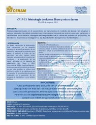
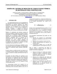
En <strong>la</strong> Figura 1 se presenta <strong>la</strong> comparación <strong>de</strong> <strong>la</strong><br />
<strong>incertidumbre</strong> <strong>expandida</strong>, obtenida <strong>de</strong> acuerdo a<br />
(12), por no consi<strong>de</strong>rar <strong>los</strong> <strong>grados</strong> <strong>de</strong> <strong>libertad</strong> y<br />
expan<strong>de</strong>r con k = 2 (M1), con el método<br />
recomendado por <strong>la</strong> GUM, dada por <strong>la</strong> razón:<br />
1,0<br />
0,8<br />
0,6<br />
0,4<br />
0,2<br />
0,0<br />
2 ⋅ u<br />
U<br />
c<br />
=<br />
t<br />
2 ⋅ u<br />
( ν<br />
c<br />
) ⋅ u<br />
=<br />
t<br />
2<br />
( ν<br />
95% 95,<br />
45 ef c 95,<br />
45 ef<br />
uA = uB<br />
)<br />
(15)<br />
Fig. 1 Incertidumbre <strong>expandida</strong> como función <strong>de</strong> uA y<br />
para diferentes valores νA , obtenida con M1 y<br />
normalizada con respecto al método recomendado por <strong>la</strong><br />
GUM.<br />
1,0<br />
0,8<br />
0,6<br />
0,4<br />
0,2<br />
0,0<br />
Incertidumbre <strong>expandida</strong> - M1 : U 1 / U 95%<br />
0,0 0,1 0,2 0,3 0,4 0,5 0,6 0,7 0,8 0,9 1,0 u A<br />
Incertidumbre <strong>expandida</strong> - M1 : U 1 / U 95%<br />
u A /u B<br />
0 2 4 6 8 10 12 14 16 18 20 ν A<br />
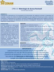
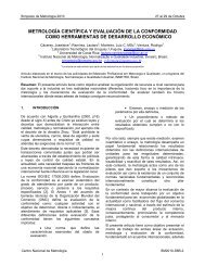
Fig. 2 Incertidumbre <strong>expandida</strong> como función <strong>de</strong> νA<br />
y para diferentes razones uA /uB , obtenida con M1 y<br />
v A<br />
15<br />
10<br />
7<br />
5<br />
3<br />
2<br />
1<br />
0,5<br />
1<br />
2<br />
inf.
normalizada con respecto al método recomendado por <strong>la</strong><br />
GUM. La última curva (“inf.”) significa que uB=0.<br />
Como se esperaba, se observa una subestimación<br />
consi<strong>de</strong>rable en el caso <strong>de</strong> una contribución<br />
dominante <strong>de</strong> uA con pocos <strong>grados</strong> <strong>de</strong> <strong>libertad</strong>.<br />
De forma simi<strong>la</strong>r, <strong>la</strong> Figura 2 muestra esta subestimación<br />
por M1 en función <strong>de</strong>l número efectivo<br />
<strong>de</strong> <strong>grados</strong> <strong>de</strong> <strong>libertad</strong>, para diferentes razones uA<br />
/uB.<br />
1,6<br />
1,4<br />
1,2<br />
1<br />
0,8<br />
0,6<br />
0,4<br />
1,3<br />
1,2<br />
1,1<br />
1<br />
0,9<br />
0,8<br />
0,7<br />
0,6<br />
1,2<br />
1,1<br />
1<br />
0,9<br />
0,8<br />
0,7<br />
Incertidumbre <strong>expandida</strong> U x / U 95% - v A = 2<br />
0 0,1 0,2 0,3 0,4 0,5 0,6 0,7 0,8 0,9 1 u A<br />
Incertidumbre <strong>expandida</strong> U x / U 95% - v A = 3<br />
0 0,1 0,2 0,3 0,4 0,5 0,6 0,7 0,8 0,9 1 u A<br />
Incertidumbre <strong>expandida</strong> U x / U 95% - v A = 7<br />
0 0,1 0,2 0,3 0,4 0,5 0,6 0,7 0,8 0,9 1<br />
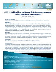
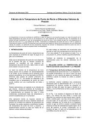
Fig. 3 Incertidumbre <strong>expandida</strong> como función <strong>de</strong> uA para<br />
νA = 2, 3 y 7 obtenida con <strong>los</strong> cuatro métodos y<br />
normalizada con respecto al método recomendado por <strong>la</strong><br />
GUM. La línea vertical a uA=0,71 indica <strong>la</strong> igualdad uA=uB<br />
M1<br />
M2<br />
M3<br />
M4<br />
M1<br />
M2<br />
M3<br />
M4<br />
M1<br />
M2<br />
M3<br />
M4<br />
para este valor.Las discontinuida<strong>de</strong>s (escalones) en<br />
<strong>la</strong>s gráficas resultan <strong>de</strong> un truncamiento <strong>de</strong> <strong>los</strong><br />
valores exactos obtenidos para vef.<br />
La Figura 3 muestra una comparación <strong>de</strong> diferentes<br />
métodos Ux con el método recomendado por <strong>la</strong><br />
GUM U95% para νA = 2, 3 y 7, presentando <strong>la</strong> razón<br />
U x U 95%<br />
. Valores mayores a 1 significan una<br />
sobreestimación <strong>de</strong> <strong>la</strong> <strong>incertidumbre</strong>, mientras<br />
valores menores a 1 significan una subestimación.<br />
Se observa que M2 siempre resulta en una<br />
sobreestimación, mientras M3 resulta en una<br />
subestimación si uA es mayor <strong>de</strong> uB . Esta<br />
subestimación pue<strong>de</strong> ser bastante gran<strong>de</strong>, para νA<br />
pequeño y u A >> uB<br />
. Sin embargo, M3 da mejores<br />
resultados que M1 (o sea sin corrección por <strong>los</strong><br />
<strong>grados</strong> <strong>de</strong> <strong>libertad</strong>).<br />
El M4 muestra un comportamiento parecido a M2,<br />
salvo en el caso <strong>de</strong> una dominancia <strong>de</strong> uB. En este<br />
caso, pue<strong>de</strong> subestimar <strong>la</strong> <strong>incertidumbre</strong> hasta 13%,<br />
si u B >> u A (ver también [1], G.5.2).<br />
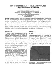
Fig. 4 Incertidumbre <strong>expandida</strong> como función <strong>de</strong> uA y<br />
para diferentes valores νA , obtenida con M2 y<br />
normalizada con respecto al método recomendado por <strong>la</strong><br />
3,6<br />
3,4<br />
3,2<br />
3<br />
2,8<br />
2,6<br />
2,4<br />
2,2<br />
2<br />
1,8<br />
1,6<br />
1,4<br />
1,2<br />
1<br />
0,8<br />
GUM.<br />
Incertidumbre <strong>expandida</strong> - M2 : U 2 / U 95%<br />
0 0,1 0,2 0,3 0,4 0,5 0,6 0,7 0,8 0,9 1 u A<br />
v A<br />
1<br />
2<br />
3<br />
5<br />
7<br />
10
Para el caso extremo <strong>de</strong> νA = 1 <strong>la</strong> sobreestimación<br />
por M2 y M4 llega hasta un factor 3,5 (para<br />
u A ≈ u B,<br />
ver Figura 4) y <strong>la</strong> subestimación por M3 y<br />
M1 llega hasta 86%.<br />
Para νA gran<strong>de</strong>s, todos <strong>los</strong> métodos se acercan<br />
cada vez más al método recomendado por <strong>la</strong> GUM.<br />
La Figura 4 muestra este comportamiento para M2<br />
variando νA<br />
CONCLUSIONES<br />
Los resultados presentados se pue<strong>de</strong>n resumir en<br />
<strong>la</strong>s siguientes conclusiones:<br />
1) No consi<strong>de</strong>rar <strong>los</strong> <strong>grados</strong> <strong>de</strong> <strong>libertad</strong> en el<br />
cálculo <strong>de</strong> <strong>la</strong> <strong>incertidumbre</strong> <strong>expandida</strong> en M1<br />
resulta en una subestimación notable,<br />
so<strong>la</strong>mente cuando uA es dominante y tiene<br />
pocos <strong>grados</strong> <strong>de</strong> <strong>libertad</strong>.<br />
2) M3 da una subestimación <strong>de</strong> <strong>la</strong> <strong>incertidumbre</strong><br />
<strong>expandida</strong> cuando uA supera uB , que pue<strong>de</strong> ser<br />
gran<strong>de</strong> si uA es dominante y tiene pocos <strong>grados</strong><br />
<strong>de</strong> <strong>libertad</strong>.<br />
3) M2 siempre sobreestima <strong>la</strong> <strong>incertidumbre</strong><br />
<strong>expandida</strong> y pue<strong>de</strong> ser consi<strong>de</strong>rada como un<br />
“método conservador”. La sobreestimación<br />
generalmente es mo<strong>de</strong>rada (menor <strong>de</strong> 22%),<br />
salvo en <strong>los</strong> casos <strong>de</strong><br />
a) νA = 1<br />
b) νA = 2 y <strong>la</strong>s contribuciones <strong>de</strong> uA y uB son<br />
parecidas<br />
4) M4 da resultados parecidos a M2, con<br />
<strong>de</strong>sviaciones <strong>de</strong> éste (subestimación <strong>de</strong> <strong>la</strong><br />
<strong>incertidumbre</strong> <strong>expandida</strong>) en el caso <strong>de</strong> que<br />
domine uB .<br />
Se resume que ninguno <strong>de</strong> <strong>los</strong> métodos analizados<br />
representa una aproximación muy cercana al<br />
método recomendado por <strong>la</strong> GUM. Todos <strong>los</strong><br />
métodos simplificados, salvo M2, pue<strong>de</strong>n presentar<br />
subestimaciones <strong>de</strong> <strong>la</strong> <strong>incertidumbre</strong>, lo que por sí<br />
pue<strong>de</strong> ser crítico. En algunos casos y <strong>de</strong>ntro <strong>de</strong><br />
ciertos límites, p. ej. uA obtenido a partir <strong>de</strong> por lo<br />
menos n = 3 mediciones, pue<strong>de</strong>n ser aceptados<br />
como aproximaciones, cuando <strong>los</strong> resultados <strong>de</strong> <strong>la</strong><br />
estimación <strong>de</strong> <strong>la</strong> <strong>incertidumbre</strong> no son sumamente<br />
críticos. Esto vale, por ejemplo, cuando el daño<br />
provocado por una medición equivocada no es muy<br />
alto, o cuando <strong>los</strong> resultados <strong>de</strong> <strong>la</strong>s mediciones no<br />
se encuentran cerca <strong>de</strong> <strong>la</strong>s tolerancias <strong>de</strong>l producto<br />
medido (verificado).<br />
Sin embargo, hay que cuestionar <strong>la</strong>s ventajas <strong>de</strong> <strong>la</strong><br />
simplificación <strong>de</strong> M2, M3 y M4, que, <strong>de</strong> todas<br />
maneras, requieren conocimientos <strong>de</strong>l metrólogo<br />
sobre <strong>los</strong> <strong>grados</strong> <strong>de</strong> <strong>libertad</strong>. Utilizando hojas <strong>de</strong><br />
cálculo para el análisis <strong>de</strong> <strong>los</strong> resultados, como p.<br />
ej. Excel, el cálculo <strong>de</strong>l número efectivo <strong>de</strong> <strong>los</strong><br />
<strong>grados</strong> <strong>de</strong> <strong>libertad</strong> pue<strong>de</strong> ser automatizado, así que<br />
el método recomendado por <strong>la</strong> GUM realmente no<br />
representa una complicación significativa en<br />
comparación con M2, M3 y M4, pero tiene <strong>la</strong><br />
ventaja <strong>de</strong> ser el método recomendado por un<br />
documento reconocido como <strong>la</strong> referencia<br />
internacional en <strong>la</strong> estimación <strong>de</strong> <strong>la</strong> <strong>incertidumbre</strong><br />
<strong>de</strong> medición.<br />
AGRADECIMIENTOS<br />
El autor quiere agra<strong>de</strong>cer a Héctor González,<br />
CENAM, por valiosas discusiones.<br />
REFERENCIAS<br />
[1] a) Gui<strong>de</strong> to the Expression of Uncertainty in<br />
Measurement, ISO 1995<br />
b) Versión traducida al español: J. M.<br />
Figueroa, Guia BIPM/ISO para <strong>la</strong> expresión<br />
<strong>de</strong> <strong>la</strong> <strong>incertidumbre</strong> en <strong>la</strong>s mediciones, CNM-<br />
MED-PT-002, CENAM 1997<br />
[2] W. Schmid, R. Lazos, Guía para estimar <strong>la</strong><br />
<strong>incertidumbre</strong> <strong>de</strong> <strong>la</strong> medición, CNM-INC-PT-<br />
001, CENAM 2000<br />
[3] ISO/TR 14353-2:1999(E), Geometrical<br />
product specification (GPS) – Inspection by<br />
measurement of workpieces and measuring<br />
equipment, Part 2<br />
[4] F. Motolonía, Cálculo <strong>de</strong> <strong>incertidumbre</strong> en<br />
calibración <strong>de</strong> indicadores <strong>de</strong> carátu<strong>la</strong>,<br />
Boletín CIDESI, 1/99, 1999, p.3<br />
[5] C. Hentschel, A. Gerster, Setting up a<br />
Calibration System for Optical Power Meters<br />
and Attenuators – A Recommendation,<br />
Hawlett Packard, Solution Note 153-2, 1996<br />
[6] Comunicación personal con varios<br />
metrólogos <strong>de</strong>l CENAM