universidad de chile facultad de ciencias físicas y matem´aticas ...
universidad de chile facultad de ciencias físicas y matem´aticas ...
universidad de chile facultad de ciencias físicas y matem´aticas ...

You also want an ePaper? Increase the reach of your titles
YUMPU automatically turns print PDFs into web optimized ePapers that Google loves.
UNIVERSIDAD DE CHILE<br />
FACULTAD DE CIENCIAS FÍSICAS Y MATEMÁTICAS<br />
DEPARTAMENTO DE INGENIERÍA MATEMÁTICA<br />
COMPLEJIDAD TOPOLÓGICA DE NILSISTEMAS Y APLICACIONES<br />
MEMORIA PARA OPTAR AL TÍTULO DE INGENIERO CIVIL MATEMÁTICO<br />
SEBASTIÁN ANDRÉS DONOSO FUENTES.<br />
PROFESOR GU ÍA:<br />
ALEJANDRO MAASS SEP ÚLVEDA<br />
PROFESOR CO-GU ÍA:<br />
MICHAEL SCHRAUDNER<br />
MIEMBROS DE LA COMISIÓN: SERVET MARTÍNEZ AGUILERA<br />
SANTIAGO DE CHILE<br />
JULIO 2011
RESUMEN DE LA MEMORIA<br />
PARA OPTAR AL TÍTULO DE<br />
INGENIERO CIVIL MATEMÁTICO POR: SEBASTIÁN DONOSO FUENTES<br />
FECHA: 13/07/2011<br />
PROF. GUIA: ALEJANDRO MAASS<br />
“COMPLEJIDAD TOPOLÓGICA DE NILSISTEMAS Y APLICACIONES”<br />
El presente trabajo <strong>de</strong> memoria tiene por objetivo principal el estudio <strong>de</strong> propieda<strong>de</strong>s<br />
topológicas <strong>de</strong> la clase <strong>de</strong> sistemas dinámicos llamados nilsistemas. Esta clase <strong>de</strong> sistemas<br />
dinámicos ha ganado importancia <strong>de</strong>s<strong>de</strong> la <strong>de</strong>mostración dada por B. Host y B. Kra en<br />
[25] <strong>de</strong> la convergencia <strong>de</strong> algunas medias ergódicas no convencionales. A partir <strong>de</strong> su<br />
<strong>de</strong>mostración se han encontrado aplicaciones importantes <strong>de</strong> los nilsistemas en Teoría<br />
Ergódica y se han <strong>de</strong>sarrollado herramientas ergódicas en otras áreas <strong>de</strong> las matemáticas,<br />
como en Combinatoria Aditiva.<br />
En su artículo Host y Kra <strong>de</strong>sarrollaron una teoría <strong>de</strong> nilsistemas <strong>de</strong>s<strong>de</strong> el contexto<br />
medible. El <strong>de</strong>sarrollo topológico <strong>de</strong> los nilsistemas se ha profundizado en dos artículos<br />
recientes <strong>de</strong> B. Host, B. Kra y A. Maass y <strong>de</strong> S. Shao y X. Ye, en 2010, en don<strong>de</strong> <strong>de</strong>muestran<br />
que cada sistema dinámico tiene factores que son nilsistemas <strong>de</strong> cualquier or<strong>de</strong>n. En esta<br />
memoria, se estudian algunas propieda<strong>de</strong>s topológicas adicionales <strong>de</strong> los nilsistemas, en<br />
particular propieda<strong>de</strong>s <strong>de</strong> mezcla y estabilización <strong>de</strong> esos factores.<br />
La complejidad asociada a un cubrimiento abierto finito en un sistema dinámico<br />
comenzó a ser estudiada en [4] en don<strong>de</strong> se muestra que esa cantidad goza <strong>de</strong> propieda<strong>de</strong>s<br />
que permiten caracterizar sistemas dinámicos. Una <strong>de</strong> las motivaciones <strong>de</strong> la presente<br />
memoria es indagar qué otros tipos <strong>de</strong> conclusiones pue<strong>de</strong>n ser obtenidas estudiando esta<br />
cantidad. Una pregunta interesante es qué clase <strong>de</strong> sistemas tiene complejidad polinomial.<br />
En particular, se estudia la complejidad <strong>de</strong> los nilsistemas y se concluye que ésta es polinomial<br />
en cada cubrimiento abierto don<strong>de</strong> el grado <strong>de</strong>l polinomio es una constante <strong>de</strong>l<br />
sistema.<br />
En el Capítulo 1 se introduce el tema <strong>de</strong> memoria, el contexto histórico matemático<br />
que la motiva y las preguntas relevantes que se <strong>de</strong>sarrollan a lo largo <strong>de</strong>l texto.<br />
En el Capítulo 2 se introducen las nociones básicas <strong>de</strong> Dinámica Topológica y Teoría<br />
Ergódica y también las <strong>de</strong>finiciones y resultados recientes relacionados con la teoría <strong>de</strong><br />
nilsistemas.<br />
En el Capítulo 3, se estudia la complejidad topológica <strong>de</strong> los nilsistemas y <strong>de</strong> sus<br />
límites inversos y se logra <strong>de</strong>mostrar que ésta es polinomial en cada cubrimiento abierto.<br />
En el Capítulo 4 se <strong>de</strong>sarrollan algunas propieda<strong>de</strong>s topológicas sobre nilsistemas, las<br />
cuales fueron obtenidas en [10] en un artículo en colaboración. Se <strong>de</strong>muestra un criterio<br />
<strong>de</strong> débil mezcla utilizando los cubos dinámicos y se prueba que la secuencia <strong>de</strong> nilfactores<br />
<strong>de</strong> un sistema dinámico o es estrictamente creciente o se estabiliza en un cierto nivel. Se<br />
estudia a<strong>de</strong>más la relación entre recurrencia con estructura IP con el límite inverso <strong>de</strong> los<br />
nilfactores topológicos. Se muestra que un sistema sin recurrencia estructurada IP es una<br />
extensión casi uno a uno <strong>de</strong>l límite inverso <strong>de</strong> sus nilfactores.<br />
Finalmente, en el Anexo se adjunta el artículo Infinite-step nilsystems, in<strong>de</strong>pen<strong>de</strong>nce<br />
and complexity, <strong>de</strong>ntro <strong>de</strong>l cual se inserta el trabajo realizado en esta memoria.
AGRADECIMIENTOS<br />
Quiero dar las gracias a todos mis amigos y compañeros que me acompañaron en<br />
este proceso. Agra<strong>de</strong>zco también enormemente a mis profesores guías por la confianza y<br />
paciencia <strong>de</strong>positada en mí, pero por sobre todo agra<strong>de</strong>zco a mis padres Javier e Iris por<br />
su apoyo incondicional durante estos años.
Índice general<br />
1. Introducción 1<br />
2. Preliminares 4<br />
2.1. Definiciones básicas en Dinámica Topológica y Teoría Ergódica . . . . . . . 4<br />
2.1.1. Sistemas Dinámicos Topológicos . . . . . . . . . . . . . . . . . . . . 4<br />
2.1.2. Semigrupo envolvente . . . . . . . . . . . . . . . . . . . . . . . . . . 6<br />
2.1.3. Factores y conjugaciones entre sistemas dinámicos topológicos . . . 7<br />
2.1.4. Sistemas Dinámicos Abstractos . . . . . . . . . . . . . . . . . . . . 8<br />
2.2. Noción <strong>de</strong> cubo y cubos dinámicos . . . . . . . . . . . . . . . . . . . . . . 9<br />
2.2.1. Cubos . . . . . . . . . . . . . . . . . . . . . . . . . . . . . . . . . . 9<br />
2.2.2. Cubos dinámicos . . . . . . . . . . . . . . . . . . . . . . . . . . . . 10<br />
2.3. Propieda<strong>de</strong>s básicas <strong>de</strong> Grupos <strong>de</strong> Lie . . . . . . . . . . . . . . . . . . . . . 12<br />
2.3.1. Campos vectoriales y el Algebra <strong>de</strong> Lie . . . . . . . . . . . . . . . . 14<br />
2.4. Nilvarieda<strong>de</strong>s y nilsistemas . . . . . . . . . . . . . . . . . . . . . . . . . . . 15<br />
2.5. Las relaciones <strong>de</strong> proximalidad regional . . . . . . . . . . . . . . . . . . . . 19<br />
2.6. Nilfactores medibles, medidas y seminormas HK . . . . . . . . . . . . . . . 21<br />
2.6.1. Construcción <strong>de</strong> factores característicos . . . . . . . . . . . . . . . . 22<br />
3. Complejidad topológica <strong>de</strong> nilsistemas 26<br />
3.1. Complejidad en un sistema dinámico topológico . . . . . . . . . . . . . . . 26<br />
3.2. Complejidad topológica en nilsistemas . . . . . . . . . . . . . . . . . . . . 29<br />
4. Sistemas Z∞<br />
4.1. La relación RP [∞] . . . . . . . . . . . . . . . . . . . . . . . . . . . . . . . . 39<br />
4.2. Complejidad y sistemas Z∞ . . . . . . . . . . . . . . . . . . . . . . . . . . 40<br />
4.3. Estabilización <strong>de</strong> nilfactores . . . . . . . . . . . . . . . . . . . . . . . . . . 40<br />
4.4. Pares <strong>de</strong> in<strong>de</strong>pen<strong>de</strong>ncia y sistemas Z∞ . . . . . . . . . . . . . . . . . . . . 44<br />
5. Conclusiones y Preguntas Abiertas 48<br />
Anexo 52<br />
iv<br />
39
Capítulo 1<br />
Introducción<br />
El estudio sistemático <strong>de</strong> sistemas dinámicos a través <strong>de</strong> sus factores fue propuesto en<br />
los 60’ en los trabajos <strong>de</strong> Furstenberg, quien notó la riqueza teórica <strong>de</strong> este concepto y las<br />
herramientas que entrega para enten<strong>de</strong>r un sistema dinámico. Variadas clases <strong>de</strong> factores<br />
han sido <strong>de</strong>scritas, tanto en el contexto medible como en el topológico. Por mencionar un<br />
ejemplo importante, en Teoría Ergódica, el factor <strong>de</strong> Kronecker es el factor más gran<strong>de</strong> que<br />
consiste en una rotación en un grupo abeliano compacto, y probar el Teorema Ergódico<br />
<strong>de</strong> Von Neumann en estos factores es suficiente para <strong>de</strong>mostrarlo en el caso general. Esta<br />
i<strong>de</strong>a se <strong>de</strong>nomina técnica <strong>de</strong> factores característicos, introducida por Furstenberg en [12].<br />
Un teorema notable <strong>de</strong> Combinatoria Aditiva <strong>de</strong>mostrado por Szemerédi [37] en un<br />
artículo publicado en 1975, afirma que cualquier subconjunto <strong>de</strong> los naturales con <strong>de</strong>nsidad<br />
superior positiva contiene progresiones aritméticas <strong>de</strong> largo arbitrario. Las herramientas<br />
usadas en esta <strong>de</strong>mostración son combinatoriales, <strong>de</strong> la teoría <strong>de</strong> grafos. Posteriormente,<br />
Furstenberg logró <strong>de</strong>mostrar este mismo resultado usando técnicas <strong>de</strong> la Teoría Ergódica,<br />
en particular un Teorema Ergódico:<br />
Teorema 1.1 (Furstenberg). Sea (X, X , µ, T ) un sistema dinámico abstracto y sea A ∈ X<br />
un conjunto con medida positiva. Entonces para cada d ∈ N,<br />
lím inf<br />
N→∞<br />
1<br />
N<br />
N<br />
µ(A ∩ T −n A ∩ T −2n A ∩ . . . ∩ T −dn A) > 0.<br />
n=1<br />
Con su <strong>de</strong>mostración, Furstenberg estableció una conexión profunda entre Teoría<br />
Ergódica y Combinatoria Aditiva, que se ha alimentado <strong>de</strong> manera creciente en los últimos<br />
años. Por citar un resultado, la <strong>de</strong>mostración <strong>de</strong>l teorema <strong>de</strong> Green y Tao que afirma que<br />
los números primos contienen progresiones aritméticas <strong>de</strong> largo arbitrario surgió <strong>de</strong> esta<br />
conexión.<br />
De aquí que toman importancia los llamados Teoremas Ergódicos no Convencionales,<br />
que se formulan como sigue. Sea (X, X , µ, T ) un sistema dinámico abstracto, d ∈ N<br />
y f1, . . . , fd funciones acotadas en X. En virtud <strong>de</strong> la <strong>de</strong>mostración <strong>de</strong> Furstenberg <strong>de</strong>l<br />
Teorema <strong>de</strong> Szemerédi interesa estudiar la convergencia en L 2 (µ) (o en algún otro espacio)<br />
<strong>de</strong> expresiones <strong>de</strong> la forma<br />
N−1<br />
1 <br />
N<br />
n=0<br />
f1(T n x)f2(T 2n x) . . . fd(T dn x)
Capítulo 1<br />
El caso d = 3 con la hipótesis <strong>de</strong> total ergodicidad fue probado por Conze y Lesigne<br />
en una serie <strong>de</strong> papers ([5], [6] y [7]) y posteriormente fue <strong>de</strong>mostrado por Host y Kra<br />
en [24] en el caso general. En el caso débilmente mezclador, Furstenberg probó que para<br />
cualquier d ∈ N el límite es constante y es igual al producto <strong>de</strong> las integrales. En el<br />
caso no débilmente mezclador probar la convergencia <strong>de</strong> tales expresiones es un problema<br />
mucho más difícil, y estuvo abierto por muchos años. Finalmente, Host y Kra en [25]<br />
<strong>de</strong>mostraron:<br />
Teorema 1.2. Sea (X, X , µ, T ) un sistema dinámico abstracto con T invertible. Sea d ∈ N<br />
y sean f1, . . . , fd funciones medibles y acotadas en X. Entonces<br />
N−1<br />
1 <br />
N<br />
n=0<br />
converge en L 2 (µ) cuando N → ∞.<br />
f1(T n x)f2(T 2n x) . . . fd(T dn x)<br />
Host y Kra lograron <strong>de</strong>mostrar este teorema usando la técnica <strong>de</strong> factores característicos<br />
<strong>de</strong> Furstenberg y tales factores característicos resultaron ser nilsistemas, los cuales han<br />
sido <strong>de</strong> gran utilidad tanto en el <strong>de</strong>sarrollo <strong>de</strong> herramientas Ergódicas en Combinatoria<br />
Aditiva (por ejemplo Green y Tao en [18],[19],[20]) como en el <strong>de</strong>sarrollo <strong>de</strong> la Teoría<br />
Ergódica en sí misma.<br />
La contraparte topológica <strong>de</strong> la teoría <strong>de</strong> nilsistemas, es <strong>de</strong>cir, los nilsistemas <strong>de</strong>s<strong>de</strong><br />
la Dinámica Topológica, ha sido <strong>de</strong>sarrollada en artículos recientes (2010) <strong>de</strong> Host, Kra,<br />
Maass [27] y Shao y Ye [38]. Ellos <strong>de</strong>muestran que cada sistema dinámico topológico tiene<br />
asociados factores que son nilsistemas <strong>de</strong> cualquier or<strong>de</strong>n, introduciendo una relación <strong>de</strong><br />
equivalencia llamada <strong>de</strong> proximalidad regional <strong>de</strong> or<strong>de</strong>n d y que se <strong>de</strong>nota RP [d] . Estudiar<br />
propieda<strong>de</strong>s topológicas adicionales <strong>de</strong> los nilsistemas es una <strong>de</strong> las motivaciones importantes<br />
<strong>de</strong> la presente memoria.<br />
Otro concepto fundamental que aparece en la teoría <strong>de</strong> los sistemas dinámicos topológicos<br />
es el <strong>de</strong> clasificación. El buscar cómo se pue<strong>de</strong>n clasificar los sistemas, qué conceptos<br />
o cantida<strong>de</strong>s son útiles para discriminar si dos sistemas dinámicos tienen naturaleza distinta,<br />
ha sido un tópico frecuente en el <strong>de</strong>sarrollo <strong>de</strong> la teoría. Algunos <strong>de</strong> los conceptos<br />
más profundos y populares que han surgido son:<br />
Estudiar propieda<strong>de</strong>s <strong>de</strong> recurrencia y en particular el estudio <strong>de</strong> los tiempos <strong>de</strong><br />
retorno. Esto es, si (X, T ) es un sistema dinámico, x ∈ X y U es una vecindad <strong>de</strong><br />
x, estudiar el conjunto <strong>de</strong> tiempos <strong>de</strong> retorno {n ∈ N : T n x ∈ U}. Esta forma <strong>de</strong><br />
estudiar un sistema fue profundizada por Furstenberg y siguió siendo <strong>de</strong>sarrollada<br />
por E.Akin, E.Glasner, W.Huang, X.Ye, entre otros. Una buena referencia sobre el<br />
tema es [14].<br />
Otra manera, sistematizada también por Furstenberg en [13] es el estudio <strong>de</strong> sistemas<br />
vía joinings, don<strong>de</strong> se clasifican los sistemas estudiando disyunciones entre distintas<br />
familias. Para una revisión sobre el tema ver [9]. En [15] se pue<strong>de</strong> encontrar una<br />
fuente más extensa y <strong>de</strong>tallada.<br />
Una tercera manera <strong>de</strong> clasificación, y es la que motiva esta memoria, es la clasificación<br />
<strong>de</strong> sistemas dinámicos usando la función <strong>de</strong> complejidad. Un ejemplo, el<br />
2
Capítulo 1<br />
caso acotado, fue estudiado por F. Blanchard, B. Host y A. Maass en [4] en don<strong>de</strong><br />
prueban que los sistemas con complejidad acotada en cada cubrimiento abierto no<br />
trivial son exactamente los sistemas don<strong>de</strong> la acción es equicontinua. Surgen a este<br />
resultado preguntas naturales sobre qué otro tipo <strong>de</strong> conclusiones se pue<strong>de</strong>n obtener<br />
<strong>de</strong> un sistema estudiando la función <strong>de</strong> complejidad, o más precisamente estudiando<br />
su escala <strong>de</strong> crecimiento . ¿Pue<strong>de</strong> caracterizar otra escala <strong>de</strong> crecimiento <strong>de</strong> la complejidad<br />
alguna clase <strong>de</strong> sistemas? En particular, es interesante estudiar qué clase<br />
<strong>de</strong> sistemas tiene una complejidad que crece polinomialmente.<br />
Por otro lado, dada la importancia <strong>de</strong> los nilsistemas en el <strong>de</strong>sarrollo mo<strong>de</strong>rno <strong>de</strong> la<br />
Teoría Ergódica y Dinámica Topológica es razonable estudiar su complejidad. Como<br />
en los ejemplos básicos <strong>de</strong> nilsistemas se observa una polinomialidad <strong>de</strong> las órbitas,<br />
es natural estudiar la relación entre complejidad <strong>de</strong> nilsistemas y polinomialidad.<br />
Esta relación es uno <strong>de</strong> los ejes centrales <strong>de</strong> esta memoria, don<strong>de</strong> <strong>de</strong>mostramos que<br />
en un nilsistema la complejidad está acotada polinomialmente en cada cubrimiento<br />
abierto, don<strong>de</strong> el grado <strong>de</strong>l polinomio es constante.<br />
3
Capítulo 2<br />
Preliminares<br />
En este capítulo entregamos algunas <strong>de</strong>finiciones básicas <strong>de</strong> Dinámica Topológica y<br />
Teoría Ergódica. A<strong>de</strong>más exponemos algunos conceptos geométricos básicos en grupos <strong>de</strong><br />
Lie que son mencionados a lo largo <strong>de</strong> esta memoria.<br />
2.1. Definiciones básicas en Dinámica Topológica y<br />
Teoría Ergódica<br />
2.1.1. Sistemas Dinámicos Topológicos<br />
Un sistema dinámico topológico (X, T ) es un espacio métrico compacto X dotado<br />
<strong>de</strong> una transformación T continua y sobreyectiva <strong>de</strong> X en sí mismo. Escribiremos s.d.t.<br />
por sistema dinámico topológico o simplemente hablaremos <strong>de</strong> sistema. En esta memoria<br />
supondremos que T es un homeomorfismo.<br />
En lo que sigue mostramos algunos <strong>de</strong> los conceptos clásicos más usados en Dinámica<br />
Topológica, como la transitividad, minimalidad y débil mezcla, y teoremas ligados a estos<br />
conceptos.<br />
Un sistema dinámico topológico (X, T ) se dice transitivo si para cualquier par <strong>de</strong><br />
abiertos no vacíos U, V ⊆ X existe n ∈ N con U ∩ T −n (V ) = ∅. Se tiene,<br />
Teorema 2.1 ([1],Cap 1). Sea (X, T ) un s.d.t. Son equivalentes:<br />
1. (X, T ) es transitivo.<br />
2. Existe x ∈ X tal que orb(x)+ = {T n (x) : n ∈ N} = X.<br />
3. Existe x ∈ X tal que orb(x)− = {T n (x) : n ∈ −N} = X.<br />
4. Existe x ∈ X tal que orb(x) = {T n (x) : n ∈ Z} = X.<br />
5. {x ∈ X : orb(x) = X} es un Gδ <strong>de</strong>nso.<br />
6. Si U ⊆ X es un abierto T -invariante no vacío, entonces U es <strong>de</strong>nso en X.<br />
4
2.1. Definiciones básicas en Dinámica Topológica y Teoría Ergódica Capítulo 2<br />
Un s.d.t. (X, T ) se dice débilmente mezclador si (X × X, T × T ) es transitivo. Se tiene,<br />
Teorema 2.2 ([1], Cap 7). Son equivalentes:<br />
1. (X, T ) es débilmente mezclador.<br />
2. Para A, B, C, D ⊆ X abiertos no vacíos existe n ∈ N tal que simultáneamente<br />
A ∩ T −n (C) = ∅ y B ∩ T −n (D) = ∅.<br />
3. (X × X, T × T ) es débilmente mezclador.<br />
4. Para todo k ∈ N y (A1, · · · , Ak), (B1, · · · , Bk) k-tuplas <strong>de</strong> abiertos no vacíos existe<br />
n ∈ N tal que simultáneamente Ai ∩ T −n (Bi) = ∅ para todo i ∈ {1, . . . , k}.<br />
Una forma fuerte <strong>de</strong> transitividad es la minimalidad. Un s.d.t. (X, T ) se dice minimal si<br />
cada x ∈ X tiene órbita <strong>de</strong>nsa, es <strong>de</strong>cir orb(x) = X en cada x ∈ X. Se tiene,<br />
Teorema 2.3 ([1], Cap 1). Son equivalentes:<br />
1. (X, T ) es minimal.<br />
2. No existen conjuntos no vacíos cerrados e invariantes distintos a X.<br />
3. Para cada conjunto U abierto no vacío, se tiene <br />
T n (U) = X.<br />
4. Para cada conjunto U abierto no vacío, existe N ∈ N tal que N<br />
n∈Z<br />
n=−N<br />
T n (U) = X.<br />
5. Para cada x ∈ X y cada vecindad U <strong>de</strong> x, el conjunto N(x, U) = {n ∈ N : T n (x) ∈<br />
U} es sindético, es <strong>de</strong>cir existe K ∈ N con N(x, U) + {1, . . . , K} = Z.<br />
Mencionamos ahora los conceptos <strong>de</strong> proximalidad y distalidad que son centrales en<br />
Dinámica Topológica <strong>de</strong>s<strong>de</strong> los teoremas <strong>de</strong> Estructura <strong>de</strong> Furstenberg.<br />
Sea (X, T ) un s.d.t. Decimos que (x, y) ∈ X × X es un par proximal si<br />
ínf<br />
n∈Z d(T n x, T n y) = 0.<br />
Denotamos por P(X) los pares proximales en (X, T ). Cuando el contexto sea claro, escribiremos<br />
P en lugar <strong>de</strong> P(X). Decimos que x e y son distales si (x, y) /∈ P(X).<br />
Ligado a los conceptos anteriores aparecen clases especiales <strong>de</strong> sistemas dinámicos<br />
topológicos. Decimos que:<br />
1. (X, T ) es una isometría si se preserva la distancia, es <strong>de</strong>cir d(x, y) = d(T x, T y) en<br />
cada x, y ∈ X.<br />
2. (X, T ) es equicontinuo si para todo > 0 existe δ > 0 tal que si d(x, y) < δ entonces<br />
d(T n x, T n y) < para todo n ∈ Z.<br />
5
3. (X, T ) es distal si P(X) = X = {(x, x) : x ∈ X}, es <strong>de</strong>cir no hay pares proximales<br />
no triviales.<br />
Claramente <strong>de</strong> las <strong>de</strong>finiciones, una isometría es un sistema equicontinuo y un sistema<br />
equicontinuo es un sistema distal. A<strong>de</strong>más, cuando el sistema es equicontinuo y minimal<br />
se pue<strong>de</strong> probar que es conjugado a una isometría minimal.<br />
Citamos algunas propieda<strong>de</strong>s clásicas <strong>de</strong> los sistemas distales, que usaremos.<br />
Teorema 2.4 (Ver [1](Caps. 5 y 7)).<br />
1. El producto cartesiano <strong>de</strong> una familia finita <strong>de</strong> sistemas distales es distal.<br />
2. Si (X, T ) es un sistema distal e Y ⊆ X es un subconjunto cerrado e invariante,<br />
entonces (Y, T ) es distal.<br />
3. Un sistema transitivo y distal es minimal.<br />
4. Un factor <strong>de</strong> un sistema distal es distal.<br />
5. Sea π : X → Y un factor entre los sistemas distales (X, T ) e (Y, T ). Si (Y, T ) es<br />
minimal, entonces π es una función abierta.<br />
2.1.2. Semigrupo envolvente<br />
En esta sección revisamos la noción <strong>de</strong> semigrupo envolvente <strong>de</strong>sarrollada por Robert<br />
Ellis en la década <strong>de</strong>l 60, la cual permite estudiar un sistema dinámico topológico minimal<br />
<strong>de</strong>s<strong>de</strong> un punto <strong>de</strong> vista algebraico.<br />
Sea (X, T ) un sistema dinámico topológico. Sea X X el conjunto <strong>de</strong> funciones <strong>de</strong> X en<br />
X. Si u, v ∈ X X <strong>de</strong>notamos como uv la composición <strong>de</strong> u y v. Con esta operación X X<br />
resulta ser un semigrupo y la acción <strong>de</strong> T en X induce en X X la operación u → T u, la<br />
cual también llamaremos T . Consi<strong>de</strong>ramos en X X la topología <strong>de</strong> la convergencia puntual<br />
(es <strong>de</strong>cir la topología producto). El semigrupo envolvente o semigrupo <strong>de</strong> Ellis E(X, T )<br />
se <strong>de</strong>fine como la clausura <strong>de</strong> {T n : n ∈ Z} en X X .<br />
Se tiene que E(X, T ) con la composición <strong>de</strong> funciones resulta ser un semigrupo compacto<br />
en el cual las operaciones<br />
u → uv y u → T u<br />
son continuas para u, v ∈ E(X, T ). Notemos que (E(X, T ), T ) resulta ser un s.d.t.<br />
El semigrupo envolvente ha ayudado a caracterizar propieda<strong>de</strong>s topológicas <strong>de</strong> un<br />
sistema dinámico. A continuación enunciamos algunos <strong>de</strong> los resultados más notables.<br />
Teorema 2.5 ([1], Caps 3 y 6). Sea (X, T ) un s.d.t. y E(X, T ) su semigrupo envolvente.<br />
Entonces:<br />
1. (X, T ) es distal si y solamente si E(X, T ) es un grupo.<br />
2. (X, T ) es equicontinuo si y solamente si E(X, T ) es un grupo <strong>de</strong> homeomorfismos<br />
<strong>de</strong> X y la topología <strong>de</strong> la convergencia puntual en E(X, T ) coinci<strong>de</strong> con la topología<br />
uniforme.
2.1. Definiciones básicas en Dinámica Topológica y Teoría Ergódica Capítulo 2<br />
Un resultado importante que permite caracterizar la proximalidad usando el semigrupo<br />
envolvente es el siguiente,<br />
Teorema 2.6 ([1], Caps 3 y 6). Sea (X, T ) un s.d.t. Se tiene,<br />
1. x1, x2 ∈ X son proximales si y solamente si existe p ∈ E(X, T ) tal que px1 = px2.<br />
2. Si x ∈ X y u ∈ E(X, T ) es un i<strong>de</strong>mpotente (es <strong>de</strong>cir, un elemento que satisface<br />
u 2 = u), entonces (x, ux) ∈ P.<br />
3. Si (X, T ) es minimal, entonces (x, y) ∈ P si y solamente si existe u ∈ E(X, T )<br />
i<strong>de</strong>mpotente minimal tal que y = ux.<br />
2.1.3. Factores y conjugaciones entre sistemas dinámicos topológicos<br />
Un factor π : (X, T ) → (Y, S) es una función continua y sobreyectiva tal que S ◦ π =<br />
π ◦ T . Cuando tal función existe, diremos que (Y, S) es un factor <strong>de</strong> (X, T ) y que (X, T )<br />
es una extensión <strong>de</strong> (Y, S). Cuando π es biyectiva se dirá que es una conjugación entre<br />
(X, T ) e (Y, S) y (X, T ) e (Y, S) se dirán sistemas conjugados. Escribiremos también<br />
π : X → Y o π : (X, T ) → (Y, T ) para <strong>de</strong>notar un factor y en general la transformación<br />
se <strong>de</strong>notará siempre T .<br />
Notemos que una relación <strong>de</strong> equivalencia R ⊆ X × X cerrada y T -invariante <strong>de</strong>fine<br />
un factor πR : (X, T ) → (X/R, T ). Recíprocamente, cada factor π : X → Y <strong>de</strong>fine la<br />
relación <strong>de</strong> equivalencia cerrada y T -invariante Rπ = {(x, x ) : π(x) = π(x )}.<br />
Un joining entre X y Y es un subconjunto J ⊆ X × Y cerrado, que se proyecta en X<br />
e Y , es <strong>de</strong>cir πX(J) = X y πY (J) = Y . Cuando J = X × Y se dirá que J es un joining no<br />
trivial. Diremos que X e Y son disjuntos como sistemas, si no existen joining no trivales<br />
y se anota X⊥Y .<br />
Hay clases importantes <strong>de</strong> factores que se <strong>de</strong>finen a partir <strong>de</strong> los conceptos <strong>de</strong> distalidad<br />
y proximalidad mencionados en la sección anterior. Definimos algunos a continuación.<br />
Sea π : X → Y un factor entre sistemas dinámicos topológicos. Decimos que (X, T )<br />
es una extensión :<br />
1. Proximal si π(x) = π(y) ⇒ (x, y) ∈ P(X).<br />
2. Distal si π(x) = π(y) y x = y ⇒ (x, y) = P(X).<br />
3. Isométrica si π(x) = π(y) ⇒ d(x, y) = d(T n x, T n y) ∀n ∈ Z.<br />
4. Casi uno a uno si {x ∈ X : π −1 (π(x)) = {x}} es un conjunto Gδ <strong>de</strong>nso.<br />
Factor equicontinuo maximal<br />
En esta subsección, mostramos un ejemplo importante <strong>de</strong> factor asociado a un sistema<br />
dinámico topológico, que ha motivado importantes generalizaciones que han contribuido a<br />
recientes y notables <strong>de</strong>sarrollos en Dinámica Topológica y Teoría Ergódica. Sea π : X → Y<br />
un factor entre los s.d.t. (X, T ) e (Y, T ). Decimos que (Y, T ) es un factor equicontinuo<br />
<strong>de</strong> (X, T ) si (Y, T ) es un s.d.t. equicontinuo. Pue<strong>de</strong> haber un amplio espectro <strong>de</strong> factores<br />
equicontinuos asociados a un sistema, pero un teorema clásico afirma lo siguiente.<br />
7
2.1. Definiciones básicas en Dinámica Topológica y Teoría Ergódica Capítulo 2<br />
Teorema 2.7. Sea (X, T ) un s.d.t. Entonces existe un factor equicontinuo maximal, es<br />
<strong>de</strong>cir un factor (Y, T ) equicontinuo, tal que si (Z, T ) es un factor equicontinuo <strong>de</strong> (X, T ),<br />
entonces (Z, T ) también es factor <strong>de</strong> (Y, T ).<br />
Al factor equicontinuo maximal <strong>de</strong> (X, T ) lo anotamos (Xeq, T ). Si (Z, T ) es cualquier<br />
factor equicontinuo <strong>de</strong> (X, T ) tenemos el siguiente diagrama conmutativo:<br />
(X, T )<br />
<br />
πeq <br />
πZ <br />
<br />
<br />
(Xeq, T ) <br />
(Z, T )<br />
πeq,Z<br />
El siguiente concepto permite construir explícitamente el factor equicontinuo maximal<br />
a través <strong>de</strong> una relación <strong>de</strong> equivalencia cerrada e invariante. Esta construcción permite<br />
generalizar el concepto <strong>de</strong> factor equicontinuo maximal, como mostraremos en la sección<br />
2.5.<br />
Sea (X, T ) un s.d.t. y x, y ∈ X. Decimos que x, y son regionalmente proximales si para<br />
cada δ > 0 y para cada > 0 existen x, y ∈ X y existe n ∈ Z con d(x, x) < δ, d(y, y) < δ<br />
y d(T n (x), T n (y)) < . Escribimos RP(X) a los pares regionalmente proximales y cuando<br />
no haya confusión, los anotaremos simplemente como RP. Es un resultado clásico que en<br />
un sistema minimal RP(X) es una relación <strong>de</strong> equivalencia.<br />
En cualquier sistema dinámico topológico se pue<strong>de</strong>n <strong>de</strong>finir los factores distal y equicontinuo<br />
maximal y se <strong>de</strong>terminan por las relaciones P(X) y RP(X).<br />
Teorema 2.8 ([15]). Sea (X, T ) un s.d.t. y sean Sd y Seq las relaciones <strong>de</strong> equivalencia<br />
cerradas, T -invariantes más pequeñas que contienen a P(X) y RP(X) respectivamente.<br />
Luego Xd = (X/Sd, T ) y Xeq = (X/Seq, T ) son el factor distal y equicontinuo maximal<br />
respectivamente.<br />
Análogamente a ser factor equicontinuo maximal, ser factor distal maximal significa<br />
que si (Z, T ) es un factor distal <strong>de</strong> (X, T ), entonces (Z, T ) también es un factor <strong>de</strong> (XD, T )<br />
Se <strong>de</strong>duce que (Xeq, T ) es factor <strong>de</strong> (XD, T ).<br />
2.1.4. Sistemas Dinámicos Abstractos<br />
Un sistema dinámico abstracto (s.d.a.) (X, X , µ, T ) es un espacio <strong>de</strong> probabilidad<br />
(X, X , µ) dotado <strong>de</strong> la transformación T : X → X X -X -medible que preserva la medida,<br />
es <strong>de</strong>cir T µ(B) := µ(T −1 B) = µ(B) para todo B ∈ X . A menudo, un s.d.a. (X, X , µ, T )<br />
lo escribiremos como (X, µ, T ), omitiendo la σ-álgebra.<br />
Sea (X, µ, T ) un s.d.a. Un conjunto medible A ∈ X se dice invariante si µ(AT −1 A) =<br />
0, don<strong>de</strong> AB = (A\B)∪(B\A). El s.d.a. (X, µ, T ) se dice ergódico si no existen conjuntos<br />
invariantes no triviales, es <strong>de</strong>cir, si A ∈ X y µ(AT −1 A) = 0 entonces necesariamente<br />
µ(A) = 0 o µ(A) = 1.<br />
Si (X, µ, T ) es un s.d.a. usaremos la palabra factor con dos significados distintos:<br />
como una sub-σ-álgebra T -invariante Y <strong>de</strong> X o como un s.d.a. (Y, Y, ν, S) y una función<br />
π : X ⊆ X → Y ⊆ Y medible con µ(X ) = ν(Y ) = 1 y tal que πµ = ν y S ◦ π = π ◦ T .<br />
Se i<strong>de</strong>ntifica la σ-álgebra Y <strong>de</strong> Y con la sub-σ-álgebra invariante π −1 (Y) <strong>de</strong> X .<br />
8
2.2. Noción <strong>de</strong> cubo y cubos dinámicos Capítulo 2<br />
Relación entre s.d.t. y s.d.a.<br />
En esta memoria el objeto <strong>de</strong> estudio son los sistemas dinámicos topológicos. Sin<br />
embargo, los sistemas dinámicos abstractos aparecen como una herramienta importante<br />
en su estudio, por lo cual mostramos resultados clásicos que relacionan tales conceptos.<br />
Sea (X, T ) un s.d.t. y consi<strong>de</strong>remos la σ-algebra <strong>de</strong> Borel B(X) generada por los<br />
abiertos <strong>de</strong> X. Denotemos por M(X) el conjunto <strong>de</strong> medidas <strong>de</strong> probabilidad <strong>de</strong>finidas<br />
sobre B(X) y M(X, T ) = {µ ∈ M(X) : T µ = µ} el conjunto <strong>de</strong> medidas invariantes para<br />
T . Los siguientes teoremas clásicos ligan los s.d.t. con los s.d.a.<br />
Teorema 2.9 (Krylov-Bogolioubov). Sea (X, T ) un s.d.t. Luego M(X, T ) es no vacío.<br />
Se tienen a<strong>de</strong>más las siguientes propieda<strong>de</strong>s <strong>de</strong> M(X, T ):<br />
Teorema 2.10. Sea (X, T ) un s.d.t., luego<br />
1. M(X, T ) es un subconjunto compacto <strong>de</strong> M(X).<br />
2. M(X, T ) es convexo.<br />
3. µ ∈ M(X, T ) es un punto extremo <strong>de</strong> M(X, T ) si y solamente si (X, µ, T ) es un<br />
s.d.a. ergódico. En este caso, <strong>de</strong>cimos que µ es una medida ergódica.<br />
4. Si µ, ν ∈ M(X, T ) son dos médidas ergódicas, entonces µ = ν o µ ⊥ ν.<br />
Así, si (X, T ) es un s.d.t., siempre existe una medida invariante µ (o ergódica) que<br />
permite estudiarlo como un s.d.a.<br />
2.2. Noción <strong>de</strong> cubo y cubos dinámicos<br />
2.2.1. Cubos<br />
En esta sección <strong>de</strong>sarrollamos la noción <strong>de</strong> cubo, introducida en [27], la cual ha sido <strong>de</strong><br />
gran utilidad en <strong>de</strong>sarrollos recientes en Dinámica Topológica y Teoría Ergódica, siendo<br />
la base <strong>de</strong> un importante Teorema <strong>de</strong> Estructura <strong>de</strong>mostrado en [27] que mencionamos al<br />
final <strong>de</strong> la Sección 2.4.<br />
Sea X un conjunto y d ∈ N. Escribimos [d] = {1, . . . , d}. Vemos el hipercubo {0, 1} d<br />
<strong>de</strong> dos maneras, como una secuencia = 1 . . . d <strong>de</strong> ceros y unos o como un subconjunto<br />
<strong>de</strong> [d]. Un subconjunto correspon<strong>de</strong> a la secuencia 1 . . . d ∈ {0, 1} d tal que i = 1 si y<br />
solamente si i ∈ . Por ejemplo 0 = 0 . . . 0 correspon<strong>de</strong> al conjunto vacío.<br />
Si n = (n1, . . . , nd) ∈ Z d y ⊂ [d], <strong>de</strong>finimos<br />
n · =<br />
d<br />
ini = <br />
ni.<br />
i=1<br />
Denotamos X [d] = X2d. Un punto x ∈ X [d] pue<strong>de</strong> ser escrito <strong>de</strong> dos maneras equivalentes,<br />
<strong>de</strong>pendiendo <strong>de</strong>l contexto,<br />
i∈<br />
x = (x : ∈ {0, 1} d ) = (x : ⊆ [d]).<br />
9
2.2. Noción <strong>de</strong> cubo y cubos dinámicos Capítulo 2<br />
Como ejemplos, los puntos en X [2] se escriben como<br />
y puntos en X [3] son <strong>de</strong> la forma<br />
(x00, x10, x01, x11) = (xφ, x{1}, x{2}, x{1,2}),<br />
(x000, x100, x010, x110, x001, x101, x011, x111) = (x∅, x{1}, x{2}, x{1,2}, x{3}, x{1,3}, x{2,3}, x{1,2,3}).<br />
Dado x ∈ X, escribimos x [d] = (x, . . . , x) ∈ X [d] . La diagonal <strong>de</strong> X [d] es [d] = {x [d] : x ∈<br />
X}.<br />
Un punto x ∈ X [d] pue<strong>de</strong> ser <strong>de</strong>scompuesto como x = (x , x ) con x , x ∈ X [d−1] ,<br />
don<strong>de</strong> x = (x0 : ∈ {0, 1} d−1 ) y x = (x1 : ∈ {0, 1} d−1 ). También po<strong>de</strong>mos aislar la<br />
primera coor<strong>de</strong>nada, escribiendo un punto x ∈ X [d] como x = (x∅, x∗), don<strong>de</strong> x∗ = (x :<br />
⊂ [d] \ {∅}) ∈ X [d]<br />
∗ := X 2d −1 .<br />
I<strong>de</strong>ntificando {0, 1} d con los vértices <strong>de</strong>l cubo unitario eucli<strong>de</strong>ano, una isometría eucli<strong>de</strong>ana<br />
<strong>de</strong>l cubo permuta los vértices <strong>de</strong>l cubo y por lo tanto las coor<strong>de</strong>nadas <strong>de</strong> x ∈ X [d] .<br />
Estas permutaciones se <strong>de</strong>nominan permutaciones eucli<strong>de</strong>anas <strong>de</strong> X [d] . Como ejemplos <strong>de</strong><br />
permutaciones eucli<strong>de</strong>anas po<strong>de</strong>mos mencionar:<br />
Permutaciones <strong>de</strong> dígitos: son las permutaciones <strong>de</strong> {0, 1} d inducidas por permutaciones<br />
<strong>de</strong> [d].<br />
Simetrías: son las permutaciones <strong>de</strong> {0, 1} d que se forman al reemplazar i por 1−i<br />
para algún i ∈ [d].<br />
Por ejemplo,<br />
(00, 10, 01, 11) → (00, 01, 10, 11)<br />
(00, 10, 01, 11) → (10, 00, 11, 01)<br />
correspon<strong>de</strong>n a una permutación <strong>de</strong> las coor<strong>de</strong>nadas y a una simetría en la primera posición.<br />
Las permutaciones eucli<strong>de</strong>anas son formadas por composiciones <strong>de</strong> permutaciones y<br />
simetrías.<br />
2.2.2. Cubos dinámicos<br />
En esta sección mostramos como formar cubos utilizando la dinámica <strong>de</strong> un sistema<br />
dinámico topológico. Esta construcción, como veremos más a<strong>de</strong>lante, pue<strong>de</strong> <strong>de</strong>cir muchas<br />
propieda<strong>de</strong>s <strong>de</strong>l sistema dinámico mismo.<br />
Sea (X, T ) un sistema dinámico topológico y d ∈ N. Definimos Q [d] (X) como la cerradura<br />
en X [d] <strong>de</strong> elementos <strong>de</strong> la forma:<br />
(T n· (x) : = (1, . . . , d) ∈ {0, 1} d )<br />
don<strong>de</strong> n = (n1, . . . , nd) ∈ Z d y x ∈ X. Cuando no haya ambiguedad escribiremos Q [d] (X)<br />
simplemente como Q [d] . Un elemento en Q [d] (X) se llamará un cubo o paralelepípedo<br />
dinámico. Observemos algunas propieda<strong>de</strong>s básicas <strong>de</strong> Q [d] (X):<br />
10
2.2. Noción <strong>de</strong> cubo y cubos dinámicos Capítulo 2<br />
1. x [d] ∈ Q [d] (X) para todo x ∈ X;<br />
2. Q [d] (X) es invariante bajo permutaciones eucli<strong>de</strong>anas;<br />
3. Si x ∈ Q [d] (X), entonces (x, x) ∈ Q [d+1] (X).<br />
Para clarificar:<br />
Q [1] (X) es la clausura en X [1] = X 2 <strong>de</strong>l conjunto {(x, T n (x)) : x ∈ X, n ∈ Z}. Si<br />
(X, T ) es minimal, Q [1] (X) = X × X.<br />
Q [2] (X) es la clausura en X [2] = X 4 <strong>de</strong>l conjunto<br />
{(x, T m x, T n x, T n+m x) : x ∈ X, n, m ∈ Z}.<br />
Q [3] (X) es la clausura en X [3] = X 8 <strong>de</strong>l conjunto<br />
{(x, T m x, T n x, T n+m x, T p x, T p+m x, T p+n x, T p+n+m x) : x ∈ X, n, m, p ∈ Z}.<br />
Si π : X → Y es un factor entre los s.d.t., (X, T ) e (Y, T ) entonces π [d] (Q [d] (X)) =<br />
Q [d] (Y ) don<strong>de</strong> π [d] = π × π · · · × π (2 d veces).<br />
Definimos a continuación transformaciones <strong>de</strong> Q [d] (X) en sí mismo, <strong>de</strong>finidas a partir<br />
<strong>de</strong> la transformación T en X, que <strong>de</strong>terminan una dinámica en Q [d] (X).<br />
Definición 2.11 (Transformaciones <strong>de</strong> fase). Sea (X, T ) un s.d.t. y d ∈ N. Definimos la<br />
transformación diagonal como T [d] : X [d] → X [d] don<strong>de</strong><br />
(T [d] x) = T x<br />
para x = (x) ∈{0,1} d .<br />
Por ejemplo, en X [2] , T [2] (x00, x10, x01, x11) = (T x00, T x10, T x01, T x11).<br />
Para cada j ∈ [d] <strong>de</strong>finimos la transformación <strong>de</strong> fase T [d]<br />
j : X [d] → X [d] como<br />
T [d]<br />
j x =<br />
<br />
(T [d]<br />
j x) = T x si j ∈ <br />
(T [d]<br />
j x) = x si j /∈ <br />
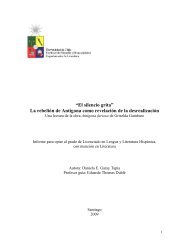
Si se piensa en las coor<strong>de</strong>nadas <strong>de</strong> x como los vértices <strong>de</strong> un cubo, estas transformaciones<br />
correspon<strong>de</strong>n a iterar la transformación en una sola cara. Por ejemplo, con k = 3, en la<br />
figura se muestran las transformaciones <strong>de</strong> fase asociadas. Cada una cambia los valores<br />
in<strong>de</strong>xados por los símbolos pintados en azul:<br />
11
x001 x110 x001 x110<br />
<br />
T<br />
x101 x111<br />
[3]<br />
<br />
<br />
1 <br />
T (x101) T (x111)<br />
x000 x010 x000 x010<br />
<br />
<br />
<br />
<br />
x100 x110<br />
T (x100) T (x110)<br />
x001 x110 x001 T (x110)<br />
<br />
T<br />
x101 x111<br />
[3]<br />
<br />
<br />
2 <br />
x101 T (x111)<br />
x000 x010 x000 T (x010)<br />
<br />
<br />
<br />
<br />
x100 x110<br />
x100 T (x110)<br />
x101<br />
x001 x110 T (x001) T (x110)<br />
<br />
<br />
x111<br />
T [3]<br />
3 <br />
T (x101)<br />
T (x111)<br />
x000 x010 x000 x010<br />
<br />
<br />
<br />
<br />
x100 x110<br />
x100 x110<br />
Figura 2.1: Transformaciones <strong>de</strong> fase en X [3] .<br />
El grupo <strong>de</strong> fase <strong>de</strong> dimensión d es el grupo F [d] (X) <strong>de</strong> transformaciones en X [d]<br />
generadas por las transformaciones <strong>de</strong> fase. El grupo paralelepípedo <strong>de</strong> dimensión d es el<br />
grupo G [d] (X) generado por la transformación diagonal y por las transformaciones <strong>de</strong> fase.<br />
Similar a la notación usada en X [d] , un elemento S ∈ F [d] (X) (o en G [d] (X)) será escrito<br />
como:<br />
S = (S : ∈ {0, 1} d } = (S : ⊆ [d]}).<br />
En particular,<br />
F [d] (X) = {S ∈ G [d] (X) : S∅ = Id}.<br />
Notamos que el grupo G [d] satisface propieda<strong>de</strong>s análogas a Q [d] :<br />
1. T [d] ∈ G [d] ;<br />
2. G [d] es invariante bajo permutaciones eucli<strong>de</strong>anas;<br />
3. Si S ∈ G [d] , entonces (S, S) ∈ G [d+1] .<br />
2.3. Propieda<strong>de</strong>s básicas <strong>de</strong> Grupos <strong>de</strong> Lie<br />
En esta memoria aparecerá como objeto <strong>de</strong> estudio el concepto <strong>de</strong> grupo <strong>de</strong> Lie, lo<br />
cual hace necesario mostrar las nociones básicas sobre Grupos <strong>de</strong> Lie que se discutirán a<br />
lo largo <strong>de</strong> este texto. Dedicaremos esta sección a tal propósito, sin ambición <strong>de</strong> entrar en<br />
mayores <strong>de</strong>talles. Una referencia general a este tema es [21].
2.3. Propieda<strong>de</strong>s básicas <strong>de</strong> Grupos <strong>de</strong> Lie Capítulo 2<br />
Un grupo <strong>de</strong> Lie G o (G, ·) es un grupo (en el sentido abstracto) que a<strong>de</strong>más es una<br />
variedad diferenciable, don<strong>de</strong> las operaciones son compatibles con la diferenciabilidad, es<br />
<strong>de</strong>cir:<br />
(g, h) → g · h := gh<br />
g → g −1<br />
son funciones diferenciables <strong>de</strong> G × G → G y <strong>de</strong> G → G respectivamente.<br />
Ejemplos:<br />
1. (R n , +) es un grupo <strong>de</strong> Lie.<br />
2. Sea GLn = {A ∈ Mn×n(R) : A es invertible } el grupo lineal general. Es una variedad<br />
n 2 -dimensional, y con la multiplicación usual <strong>de</strong> matrices resulta ser un grupo <strong>de</strong><br />
Lie. Consta <strong>de</strong> dos componentes conexas, GL + n = {A ∈ Mn×n(R) : <strong>de</strong>t(A) > 0} y<br />
GL − n = {A ∈ Mn×n(R) : <strong>de</strong>t(A) < 0}.<br />
3. Sea O(n) = {A ∈ Mn×n(R) : A T A = Id}, con la multiplicación usual <strong>de</strong> matrices.<br />
Es un grupo <strong>de</strong> Lie que se <strong>de</strong>nomina grupo ortogonal y consta <strong>de</strong> dos componentes<br />
conexas, O(n) + = {A ∈ O(n) : <strong>de</strong>t(A) = 1} y O(n) − = {A ∈ O(n) : <strong>de</strong>t(A) = −1}.<br />
4. Sea SO(n) = O(n) + = {A ∈ O(n) : <strong>de</strong>t(A) = 1} con la multiplicación usual <strong>de</strong><br />
matrices. Resulta ser un grupo <strong>de</strong> Lie conexo y se le <strong>de</strong>nomina el grupo especial<br />
ortogonal.<br />
⎧⎛<br />
⎞<br />
⎫<br />
⎨ 1 x z<br />
⎬<br />
5. Sea G = ⎝ 0 1 y ⎠ : x, y, z ∈ R con la multiplicación usual <strong>de</strong> matrices. Es<br />
⎩<br />
⎭<br />
0 0 1<br />
un grupo <strong>de</strong> Lie conexo y se <strong>de</strong>nomina el grupo <strong>de</strong> Heisenberg.<br />
6. Sea<br />
⎧⎛<br />
⎞<br />
⎫<br />
1 x1 x2 . . . xn z<br />
⎜<br />
⎪⎨<br />
⎜ 1 0 . . . 0 y1<br />
⎟<br />
⎜<br />
. ..<br />
. ..<br />
⎟<br />
⎪⎬<br />
Hn = ⎜<br />
. . ⎟ : x1, . . . , xn, y1, . . . , yn, z ∈ R<br />
⎜<br />
1 0 yn−1 ⎟<br />
⎝<br />
⎪⎩<br />
0 1 yn ⎠<br />
⎪⎭<br />
1<br />
con la multiplicación <strong>de</strong> matrices. Es un grupo <strong>de</strong> Lie y es la generalización más<br />
simple <strong>de</strong>l grupo <strong>de</strong> Heisenberg.<br />
7. Sea<br />
⎧⎛<br />
⎪⎨<br />
⎜<br />
Un = ⎜<br />
⎝<br />
⎪⎩<br />
1 a12 . . . . . . a1n<br />
1 a23 . . . a2n<br />
. ..<br />
0 1 an−1,n<br />
1<br />
13<br />
⎞<br />
⎫<br />
⎟<br />
⎪⎬<br />
⎟ : aij ∈ R si j − i ≥ 1<br />
⎟<br />
⎠<br />
⎪⎭
2.3. Propieda<strong>de</strong>s básicas <strong>de</strong> Grupos <strong>de</strong> Lie Capítulo 2<br />
con la multiplicación usual <strong>de</strong> matrices. Es un grupo <strong>de</strong> Lie y lo llamaremos el grupo<br />
<strong>de</strong> Heisenberg <strong>de</strong> or<strong>de</strong>n n.<br />
8. Sea G = R × R × S 1 = {(x, y, z) : x ∈ R, y ∈ R, z ∈ C, |z| = 1} y <strong>de</strong>finamos la<br />
operación<br />
(x1, y1, z1) ∗ (x2, y2, z2) → (x1 + x2, y1 + y2, e ix1y2 z1z2)<br />
Se pue<strong>de</strong> probar que G es un grupo <strong>de</strong> Lie y que no es isomorfo (como grupo) a<br />
ningún grupo matricial.<br />
2.3.1. Campos vectoriales y el Algebra <strong>de</strong> Lie<br />
Los siguientes conceptos y resultados geométricos son clásicos, para una referencia ver<br />
[21], [22].<br />
Sea G un grupo <strong>de</strong> Lie <strong>de</strong> dimensión m. Un campo vectorial es una función X que a<br />
cada g ∈ G le asocia Xg ∈ Tg(G) don<strong>de</strong> Tg(G) es el espacio tangente a G en g. Usando<br />
un sistema <strong>de</strong> coor<strong>de</strong>nadas, po<strong>de</strong>mos expresar el campo vectorial como<br />
<br />
m<br />
Xg(f) = ak(g) ∂f<br />
<br />
g<br />
para cada f ∈ C<br />
∂xk<br />
∞ (G).<br />
k=1<br />
Po<strong>de</strong>mos <strong>de</strong>finir una función C ∞ (G) → C ∞ (G), que llamaremos también X, escribiendo<br />
X(f)(g) = Xg(f). A X <strong>de</strong>finido <strong>de</strong> esta forma lo llamaremos también un campo<br />
vectorial. Para X e Y campos vectoriales (como funciones <strong>de</strong> C ∞ (G) en sí mismo) <strong>de</strong>finimos<br />
[X, Y ] = X ◦Y −Y ◦X. Con esta operación, los campos vectoriales forman un álgebra<br />
<strong>de</strong> Lie <strong>de</strong> dimensión infinita.<br />
Sea g ∈ G un elemento fijo y <strong>de</strong>finamos la aplicación Lg : G → G por Lg(h) = gh.<br />
Como la multiplicación es suave en G × G, Lg resulta ser diferenciable. Denotemos por<br />
D(Lg) el diferencial <strong>de</strong> Lg. Luego D(Lg)(h) : Th(G) → TLg(h)(G) = Tgh(G) es un funcional<br />
lineal. Un campo vectorial se dice invariante por la izquierda si<br />
D(Lg)(h)(Xh) = Xgh para cualquier g, h ∈ G<br />
Sea Te(G) el espacio tangente a G en la i<strong>de</strong>ntidad e y sea v ∈ Te(G). Definamos el campo<br />
vectorial Xv colocando Xv g = D(Lg)(e)(v). Éste es el único campo vectorial que satisface<br />
X v e = v. Se tiene que el espacio <strong>de</strong> campos vectoriales invariantes por la izquierda es un<br />
espacio vectorial <strong>de</strong> la misma dimensión que G y es isomorfo como espacio vectorial a Tg(e)<br />
vía evaluación en la i<strong>de</strong>ntidad. Este isomorfismo permite hacer la siguiente <strong>de</strong>finición.<br />
Definición 2.12 ( Álgebra <strong>de</strong> Lie). Sea G un grupo <strong>de</strong> Lie. El álgebra <strong>de</strong> Lie g <strong>de</strong> G es<br />
el espacio tangente a G en la i<strong>de</strong>ntidad e, dotado <strong>de</strong> la operación <strong>de</strong>finida por<br />
[v, w] = [X v , X w ](e).<br />
Sea G un grupo <strong>de</strong> Lie simplemente conexo y g = Te(G) el álgebra <strong>de</strong> Lie. Se <strong>de</strong>fine el<br />
mapeo exponencial exp : g → G como exp(v) = γ(1) don<strong>de</strong> γ es la única curva γ : R → G<br />
14
2.4. Nilvarieda<strong>de</strong>s y nilsistemas Capítulo 2<br />
tal que dγ<br />
dt |t=0 = v. Sea G 0 la componente conexa <strong>de</strong> la i<strong>de</strong>ntidad. Si G es simplemente<br />
conexo, G 0 es exponencial, es <strong>de</strong>cir el mapeo exponencial entre g y G 0 es un difeomorfismo.<br />
Luego, si G es conexo y simplemente conexo exp : g → G es un difeomorfismo.<br />
Sean G un grupo <strong>de</strong> Lie conexo y simplemente conexo y sean a = exp(X), b = exp(Y )<br />
don<strong>de</strong> a, b ∈ G y X, Y ∈ g. En este caso ab = exp(Z) para algún Z ∈ g. La pregunta<br />
natural es la relación entre Z, X e Y . Esto lo respon<strong>de</strong> la fórmula <strong>de</strong> Baker-Campbell-<br />
Hausdorff.<br />
Teorema 2.13. Sea G un grupo <strong>de</strong> Lie simplemente conexo, sean X, Y ∈ g y sea Z ∈ g<br />
tal que exp(Z) = exp(X) exp(Y ). Entonces, se tiene la siguiente fórmula<br />
don<strong>de</strong><br />
1<br />
12<br />
Z = (−1) n−1<br />
n<br />
n>0<br />
<br />
r i +s i >0<br />
1≤i≤n<br />
[X r1 Y s1 · · · X rn Y sn ] = [X, [X, . . . [X,<br />
( n<br />
i=1 ri + si) −1<br />
r1!s1! · · · rn!sn! [Xr1 Y s1 · · · X rn Y sn ]<br />
, [Y, [Y, . . . [Y, , . . . , [X, [X, . . . [X, , [Y, [Y, . . . Y ] ] . . .]<br />
<br />
r1<br />
s1<br />
Los primeros términos <strong>de</strong> la serie vienen dados por X + Y + 1<br />
1 [X, Y ] + [X, [X, Y ]] −<br />
2 12<br />
1<br />
[Y, [X, Y ]] − [Y, [X, [X, Y ]]] + . . . .<br />
24<br />
Si G es abeliano se tiene exp(X) exp(Y ) = exp(X + Y ).<br />
2.4. Nilvarieda<strong>de</strong>s y nilsistemas<br />
En esta sección <strong>de</strong>finimos las nilvarieda<strong>de</strong>s y nilsistemas, que serán los sistemas dinámicos<br />
<strong>de</strong> nuestro interés en esta memoria.<br />
Sea G un grupo y [·, ·] el conmutador asociado, es <strong>de</strong>cir [a, b] = a −1 b −1 ab en cada<br />
a, b ∈ G. Dados subgrupos A, B ⊆ G, escribimos [A, B] para <strong>de</strong>notar al subgrupo generado<br />
por {[a, b] : a ∈ A, b ∈ B}. Se <strong>de</strong>finen inductivamente los subgrupos conmutadores Gj<br />
como:<br />
G0 = G<br />
Gj+1 = [G, Gj] j ≥ 0<br />
Definición 2.14. Decimos que G es un grupo nilpotente <strong>de</strong> or<strong>de</strong>n d si Gd es el subgrupo<br />
trivial.<br />
Ejemplos:<br />
El grupo nilpotente <strong>de</strong> or<strong>de</strong>n 0 es el grupo trivial.<br />
Un grupo es nilpotente <strong>de</strong> or<strong>de</strong>n 1 si y solamente si es abeliano.<br />
El grupo <strong>de</strong> Heisenberg <strong>de</strong>finido en la Sección 2.3 es nilpotente <strong>de</strong> or<strong>de</strong>n 2.<br />
Los grupos Hn <strong>de</strong>finidos en la Sección 2.3 son nilpotentes <strong>de</strong> or<strong>de</strong>n 2.<br />
15<br />
rn<br />
sn
2.4. Nilvarieda<strong>de</strong>s y nilsistemas Capítulo 2<br />
Los grupos <strong>de</strong> Heisenberg Un <strong>de</strong>finidos en la Sección 2.3 son nilpotentes <strong>de</strong> or<strong>de</strong>n<br />
n − 1.<br />
Definición 2.15. Dado un grupo <strong>de</strong> Lie G nilpotente <strong>de</strong> or<strong>de</strong>n d y Γ un subgrupo discreto<br />
cocompacto <strong>de</strong> G (es <strong>de</strong>cir, numerable y tal que G/Γ es compacto), <strong>de</strong>cimos que X = G/Γ<br />
es una nilvariedad <strong>de</strong> or<strong>de</strong>n d. Los elementos <strong>de</strong> X se anotan como hΓ don<strong>de</strong> h ∈ G.<br />
En X consi<strong>de</strong>ramos la acción T dada por la traslación por la izquierda por un elemento<br />
g ∈ G fijo, es <strong>de</strong>cir T (hΓ) = ghΓ. El sistema (X, T ) resulta ser un s.d.t. Sea µ la medida<br />
<strong>de</strong> Haar <strong>de</strong> (X, T ) (aquella invariante por rotaciones en el grupo). Ésta es la única medida<br />
<strong>de</strong> probabilidad invariante bajo T . Notamos que (X, µ, T ) resulta ser un s.d.a. y tanto al<br />
s.d.t. (X, T ) como al s.d.a. (X, µ, T ) los llamaremos nilsistemas <strong>de</strong> or<strong>de</strong>n d o d-nilsistemas.<br />
Ejemplos:<br />
La rotación Rα : x → x + α en un grupo abeliano compacto es un nilsistema <strong>de</strong><br />
or<strong>de</strong>n 1.<br />
Sea<br />
⎧⎛<br />
⎨<br />
G = ⎝<br />
⎩<br />
1 z y<br />
0 1 x<br />
0 0 1<br />
⎞<br />
⎫<br />
⎬<br />
⎠ : x, y ∈ R, z ∈ Z<br />
⎭<br />
⎧⎛<br />
⎨<br />
Γ = ⎝<br />
⎩<br />
1 m k<br />
0 1 n<br />
0 0 1<br />
⎞<br />
⎫<br />
⎬<br />
⎠ : n, m, k ∈ Z<br />
⎭<br />
Es fácil ver que po<strong>de</strong>mos i<strong>de</strong>ntificar T2 con G/Γ asociando a (x, y) ∈ T2 ⎛ ⎞<br />
el elemento<br />
1 0 y<br />
⎝ 0 1 x ⎠ Γ.<br />
0 0 1<br />
⎛<br />
1 1<br />
⎞<br />
0<br />
Consi<strong>de</strong>remos la acción T dada por la multiplicación por g = ⎝ 0 1 α ⎠ y notemos<br />
que<br />
0 0 1<br />
⎛<br />
1 1<br />
⎞ ⎛<br />
0 1 0<br />
⎞<br />
y<br />
⎛<br />
1 1 x + y<br />
⎞ ⎛<br />
1 0 x + y<br />
⎞<br />
⎝ 0 1 α ⎠ ⎝ 0 1 x ⎠ Γ = ⎝ 0 1 x + α ⎠ Γ = ⎝ 0 1 x + α ⎠ Γ<br />
0 0 1 0 0 1 0 0 1<br />
0 0 1<br />
El sistema (G/Γ, T ) es un nilsistema <strong>de</strong> or<strong>de</strong>n 2 y se conoce como el toro torcido.<br />
El sistema <strong>de</strong> Heisenberg <strong>de</strong> or<strong>de</strong>n n, dado por (Un/Γn, T ) don<strong>de</strong><br />
⎧⎛<br />
1<br />
⎪⎨<br />
⎜<br />
Un = ⎜<br />
⎝<br />
⎪⎩<br />
a12<br />
1<br />
0<br />
. . .<br />
a23<br />
. ..<br />
. . .<br />
. . .<br />
1<br />
⎞<br />
⎫<br />
a1n<br />
a2n<br />
⎟<br />
⎪⎬<br />
⎟ : aij ∈ R si j − i ≥ 1<br />
⎟<br />
an−1,n ⎠<br />
⎪⎭<br />
1<br />
16
2.4. Nilvarieda<strong>de</strong>s y nilsistemas Capítulo 2<br />
Γn =<br />
⎧⎛<br />
⎪⎨<br />
⎜<br />
⎝<br />
⎪⎩<br />
1 m12 . . . . . . m1n<br />
1 m23 . . . m2n<br />
. ..<br />
0 1 mn−1,n<br />
1<br />
⎞<br />
⎫<br />
⎟<br />
⎪⎬<br />
⎟ : mij ∈ Z si j − i ≥ 1<br />
⎟<br />
⎠<br />
⎪⎭<br />
y T es la multiplicación por un elemento g ∈ Un, es un nilsistema <strong>de</strong> or<strong>de</strong>n n − 1.<br />
En lo que sigue mencionaremos algunas propieda<strong>de</strong>s topológicas y medibles <strong>de</strong> los nilsistemas.<br />
Teorema 2.16 ([2]). Si (G/Γ, T ) es un nilsistema, entonces es distal. Es <strong>de</strong>cir, para cada<br />
x, y ∈ X se tiene<br />
ínf<br />
n∈Z d(T n x, T n y) > 0<br />
Se observa una conexión estrecha entre la teoría medible y topológica <strong>de</strong> nilsistemas (lo<br />
que se conoce como rigi<strong>de</strong>z). Un teorema importante que exhibe este hecho es el siguiente:<br />
Teorema 2.17 ([34]). Sea (X = G/Γ, T ) un nilsistema y µ su medida <strong>de</strong> Haar. Entonces<br />
las siguientes propieda<strong>de</strong>s son equivalentes:<br />
1. (X, T ) es transitivo.<br />
2. (X, T ) es minimal.<br />
3. (X, T ) es únicamente ergódico.<br />
4. (X, µ, T ) es ergódico.<br />
Sea (X = G/Γ, µ, T ) un nilsistema <strong>de</strong> or<strong>de</strong>n d, don<strong>de</strong> T (hΓ) = ghΓ. Definimos<br />
(G/Γ)ab = G/[G, G]Γ y π : G/Γ → G/[G, G]Γ la proyección canónica. Se tiene que<br />
G/[G, G]Γ es isomorfo a R mab/Z mab don<strong>de</strong> mab = dim(G)−dim([G, G]). Sea T la rotación<br />
inducida en (G/Γ)ab por π(g). Decimos que ((G/Γ)ab, T ) es la abelianización <strong>de</strong>l nilsistema<br />
(G/Γ, T ). La importancia <strong>de</strong> la abelianización <strong>de</strong> un nilsistema viene dada por el siguiente<br />
criterio <strong>de</strong> ergodicidad.<br />
Teorema 2.18 ([2]). Sea (G/Γ, µ, T ) un nilsistema don<strong>de</strong> T es la traslación por g ∈<br />
G y sea (G/[G, G]Γ, T ) su abelianización. Supongamos que G está generado por G 0 , la<br />
componente conexa <strong>de</strong> la i<strong>de</strong>ntidad, y por el elemento g ∈ G. Luego (G/Γ, µ, T ) es ergódico<br />
si y solamente si la rotación ((G/Γ)ab, T ) es ergódica.<br />
Ejemplo:<br />
En el grupo <strong>de</strong> Heisenberg clásico<br />
⎧⎛<br />
⎞<br />
⎫ ⎧⎛<br />
⎨ 1 x z<br />
⎬ ⎨<br />
G = ⎝ 0 1 y ⎠ : x, y, z ∈ R y Γ = ⎝<br />
⎩<br />
⎭ ⎩<br />
0 0 1<br />
Es fácil ver que<br />
⎧⎛<br />
⎨<br />
[G, G] = ⎝<br />
⎩<br />
1 0 z<br />
0 1 0<br />
0 0 1<br />
17<br />
1 n k<br />
0 1 m<br />
0 0 1<br />
⎞ ⎫<br />
⎬<br />
⎠ : z ∈ R<br />
⎭<br />
⎞<br />
⎫<br />
⎬<br />
⎠ : n, m, k ∈ Z<br />
⎭ .
2.4. Nilvarieda<strong>de</strong>s y nilsistemas Capítulo 2<br />
y por lo tanto<br />
⎧⎛<br />
⎞<br />
⎫<br />
⎨ 1 n z<br />
⎬<br />
[G, G]Γ = ⎝ 0 1 m ⎠ : z ∈ R n, m ∈ Z<br />
⎩<br />
⎭<br />
0 0 1<br />
⎧⎛<br />
⎞<br />
⎫<br />
⎨ 1 x 0<br />
⎬<br />
Luego G/[G, G]Γ = ⎝ 0 1 y ⎠ : x, y ∈ [0, 1) . Si consi<strong>de</strong>ramos en G/Γ la traslación<br />
⎩<br />
⎭<br />
⎛<br />
0<br />
⎞<br />
0 1<br />
1 a c<br />
dada por g = ⎝ 0 1 b ⎠, vemos que (G/[G, G]Γ, T ) es isomorfo a (T<br />
0 0 1<br />
2 , T ) don<strong>de</strong><br />
T (x, y) = (x + a, y + b). Esta transformación es ergódica en T2 si y solamente si {1, a, b}<br />
son linealmente in<strong>de</strong>pendientes sobre Q. Como G es conexo (es homeomorfo a R3 ), concluimos<br />
que la traslación dada por g en G/Γ es ergódica si y solamente si {1, a, b} son l.i.<br />
sobre Q.<br />
Similarmente, en el grupo <strong>de</strong> Heisenberg Un <strong>de</strong> or<strong>de</strong>n n, se pue<strong>de</strong> ver que la ergodicidad<br />
<strong>de</strong>pen<strong>de</strong> <strong>de</strong> la in<strong>de</strong>pen<strong>de</strong>ncia lineal sobre Q <strong>de</strong> la superdiagonal.<br />
El caso no ergódico en general se pue<strong>de</strong> ignorar en las aplicaciones, gracias al siguiente<br />
teorema.<br />
Teorema 2.19 ([33]). Sea (G/Γ, µ, T ) un nilsistema don<strong>de</strong> T es la traslación por g ∈ G.<br />
Sea x0 ∈ G/Γ y consi<strong>de</strong>remos Y = orb(x0) = {T n x0 : n ∈ Z}. Luego, existe un subgrupo<br />
G ⊆ G tal que g ∈ G , Γ = Γ ∩ G es cocompacto en G y Y = G /Γ . Como (Y, T |Y ) es<br />
transitivo, resulta ser minimal y ergódico.<br />
En el <strong>de</strong>sarrollo <strong>de</strong> la teoría <strong>de</strong> nilsistemas son relevantes los límites inversos <strong>de</strong> éstos.<br />
La principal razón es que los límites inversos <strong>de</strong> nilsistemas no son nilsistemas, salvo si<br />
todos los grupos son abelianos.<br />
Definición 2.20 (Límites inversos secuenciales).<br />
Caso topológico:<br />
Sean {(Xi, Ti)}i∈N sistemas dinámicos topológicos don<strong>de</strong> cada Xi tiene una métrica di<br />
y diam(Xi) ≤ 1. Supongamos que existen factores πi : Xi+1 → Xi . El límite inverso <strong>de</strong><br />
estos sistemas se <strong>de</strong>fine como el conjunto<br />
X = {(xi)i∈N : πi(xi+1) = xi}<br />
el cual resulta ser un subconjunto cerrado (y por lo tanto compacto) <strong>de</strong> <br />
Xi y el cual<br />
pue<strong>de</strong> ser dotado <strong>de</strong> la métrica<br />
d(x, y) = <br />
i∈N<br />
di(xi, yi)<br />
2i .<br />
Las transformaciones (Ti)i∈N inducen en X la transformación T = <br />
Ti. Anotamos<br />
(X, T ) = lím<br />
←− (Xi, Ti).<br />
18<br />
i∈N<br />
i∈N
2.5. Las relaciones <strong>de</strong> proximalidad regional Capítulo 2<br />
Caso medible:<br />
Sean {(Xi, Xi, µi, Ti)}i∈N s.d.a. y supongamos que existen factores medibles πi : Xi+1 →<br />
Xi. Sea X el conjunto<br />
X = {(xi)i∈N : πi(xi+1) = xi}.<br />
Sea pi la proyección <strong>de</strong> X en Xi, es <strong>de</strong>cir pi((xj)j∈N) = xi. A X lo dotamos <strong>de</strong> la σ-álgebra<br />
X generada por p −1<br />
i (Xi) don<strong>de</strong> i ∈ N y con la medida µ <strong>de</strong>finida en el álgebra <br />
como µ(p −1<br />
i (B)) = µi(B) para B ∈ Xi, i ∈ N. Si T = <br />
i∈N<br />
n∈N<br />
p −1<br />
i (Xi)<br />
Ti, el límite inverso <strong>de</strong> los s.d.a.<br />
(Xi, Xi, µi, Ti) es (X, X , µ, T ) y lo anotamos (X, X , µ, T ) = lím<br />
←− (Xi, Xi, µi, Ti).<br />
Muchas propieda<strong>de</strong>s dinámicas pasan hacia el límite inverso, como minimalidad, distalidad<br />
y única ergodicidad.<br />
El siguiente teorema permite caracterizar los límites inversos <strong>de</strong> nilsistemas usando la<br />
noción <strong>de</strong> cubo dinámico.<br />
Teorema 2.21 (Teorema <strong>de</strong> Estructura (Host-Kra-Maass)). Sea (X, T ) un sistema transitivo<br />
y d ≥ 2 un entero. Las siguientes propieda<strong>de</strong>s son equivalentes:<br />
1. Si x, y ∈ Q [d] (X) tienen 2 d − 1 coor<strong>de</strong>nadas en común, entonces x = y.<br />
2. Si x, y ∈ X son tales que (x, y, . . . , y) ∈ Q [d] (X), entonces x = y.<br />
3. X es un límite inverso <strong>de</strong> nilsistemas <strong>de</strong> or<strong>de</strong>n d − 1.<br />
Un sistema satisfaciendo la hipótesis <strong>de</strong>l teorema anterior se dice un sistema <strong>de</strong> or<strong>de</strong>n<br />
(d − 1).<br />
2.5. Las relaciones <strong>de</strong> proximalidad regional<br />
En esta sección se muestran generalizaciones <strong>de</strong> la relación RP <strong>de</strong>finida anteriormente<br />
en la subsección 2.1.3. Similarmente a como RP <strong>de</strong>fine el factor equicontinuo maximal,<br />
estas relaciones <strong>de</strong>finen los nilfactores topológicos maximales que <strong>de</strong>finimos a continuación.<br />
Definición 2.22. Sea (X, T ) un s.d.t. y d ∈ N. Decimos que un factor (Y, T ) es el nilfactor<br />
<strong>de</strong> or<strong>de</strong>n d maximal si (Y, T ) es un sistema <strong>de</strong> or<strong>de</strong>n d, es factor <strong>de</strong> (X, T ) y si cada vez<br />
que existe (Z, T ) sistema <strong>de</strong> or<strong>de</strong>n d que es factor <strong>de</strong> (X, T ), (Z, T ) también es factor<br />
<strong>de</strong> (Y, T ). En caso <strong>de</strong> existir tal (Y, T ) lo escribimos como (Zd, T ) y se tiene el siguiente<br />
diagrama conmutativo.<br />
(X, T )<br />
<br />
πZ <br />
d <br />
πZ <br />
<br />
<br />
(Zd, T ) <br />
(Z, T )<br />
πZd ,Z<br />
La siguiente <strong>de</strong>finición permite construir tales factores en cualquier sistema dinámico<br />
topológico minimal.<br />
19
Definición 2.23. Sea (X, T ) un s.d.t y d ∈ N. Decimos que los puntos x, y ∈ X son<br />
regionalmente proximales <strong>de</strong> or<strong>de</strong>n d si para cualquier δ > 0, existen x , y ∈ X y un<br />
vector n = (n1, . . . , nd) ∈ Z d tales que d(x, x ) < δ, d(y, y ) < δ y<br />
don<strong>de</strong> n · = d<br />
nii.<br />
i=1<br />
d(T n· x , T n· y ) < δ ∀ ∈ {0, 1} d \ {0, . . . , 0}<br />
Denotamos por RP [d] (X) el conjunto <strong>de</strong> los pares regionalmente proximales <strong>de</strong> or<strong>de</strong>n<br />
d. Si el contexto es claro, escribiremos RP [d] en lugar <strong>de</strong> RP [d] (X).<br />
Observamos que RP [1] = RP y que para cada d ∈ N, RP [d+1] ⊆ RP [d] . Notamos<br />
también que P ⊆ RP [d] para todo d ∈ N. Damos acá una <strong>de</strong>mostración alternativa a la<br />
dada en [38], en la que usaremos la estructura <strong>de</strong> cubos. Citamos para ello el siguiente<br />
resultado <strong>de</strong> [27].<br />
Teorema 2.24. Sea (X, T ) un sistema. Luego si existe a ∈ X [d]<br />
∗ tal que (x, a, y, a) ∈ Q [d+1]<br />
entonces (x, y) ∈ RP [d] .<br />
Veamos entonces que P ⊆ RP [d−1] para cada d ≥ 2. Sean (x, y) ∈ P y d ≥ 2. En<br />
virtud <strong>de</strong>l Teorema 2.6 tomemos u i<strong>de</strong>mpotente <strong>de</strong>l semigrupo envolvente E(X, T ) tal que<br />
, j ∈ [d] asociadas a u<br />
y = ux. Consi<strong>de</strong>ramos las transformaciones <strong>de</strong> fase u [d]<br />
j<br />
u [d]<br />
j (x) =<br />
<br />
(u [d]<br />
j x) = ux si j ∈ <br />
(u [d]<br />
j x) = x si j /∈ <br />
Observamos que como Q [d] es cerrado, se tiene u [d]<br />
j (x) ∈ Q[d] si x ∈ Q [d] para todo j ∈ [d].<br />
Notamos que<br />
u [d]<br />
d (x, . . . , x) = (x, . . . , x, ux, . . . , ux) = (x, . . . , x, y, . . . , y) ∈ Q[d]<br />
u [d]<br />
d−1 (x, . . . , x, y, . . . , y) = (x, . . . , x, ux, . . . , ux, y, . . . , y, uy, . . . , uy)<br />
= (x, . . . , x, y, . . . , y, y, . . . , y, y, . . . , y)<br />
Y fácilmente <strong>de</strong>ducimos que<br />
u [d]<br />
1 ◦ u [d]<br />
2 · · · ◦ u [d]<br />
d (x[d] ) = (x, y, . . . , y) ∈ Q [d]<br />
y por lo tanto (x, y) ∈ RP [d−1] .<br />
Luego,<br />
P ⊆ . . . ⊆ RP [d+1] ⊆ RP [d] ⊆ . . . ⊆ RP [2] ⊆ RP [1] = RP.<br />
En [38], generalizando los resultados <strong>de</strong> [27], se <strong>de</strong>muestra:<br />
Teorema 2.25. Sea (X, T ) un sistema minimal y d ∈ N. Luego:<br />
1. (x, y) ∈ RP [d] si y solamente si (x, y, . . . , y) ∈ Q [d+1] si y solamente si (x, y, . . . , y) ∈<br />
F [d+1] (x [d+1] );
2. RP [d] es una relación <strong>de</strong> equivalencia;<br />
3. (X, T ) es un sistema <strong>de</strong> or<strong>de</strong>n d si y solamente si RP [d] (X) = X.<br />
Teorema 2.26. Sea π : (X, T ) → (Y, T ) un factor y d ∈ N. Luego<br />
1. (π × π)(RP [d] (X)) ⊆ RP [d] (Y ).<br />
2. Si (X, T ) es minimal, (π × π)(RP [d] (X)) = RP [d] (Y ).<br />
3. Si (X, T ) es minimal, (Y, T ) es un sistema <strong>de</strong> or<strong>de</strong>n d si y solamente si RP [d] (X) ⊆<br />
Rπ = {(x, x ) ∈ X × X : π(x) = π(x )}.<br />
En particular (X/RP [d] , T ) es el nilfactor maximal <strong>de</strong> or<strong>de</strong>n d y obtenemos el siguiente<br />
diagrama conmutativo:<br />
(X, T ) <br />
<br />
<br />
<br />
<br />
<br />
<br />
<br />
<br />
<br />
<br />
<br />
<br />
<br />
<br />
<br />
<br />
<br />
<br />
<br />
<br />
<br />
<br />
<br />
<br />
πD<br />
<br />
<br />
<br />
<br />
<br />
<br />
<br />
<br />
<br />
<br />
<br />
<br />
<br />
<br />
<br />
<br />
<br />
πeq<br />
πd+1 <br />
<br />
<br />
<br />
<br />
<br />
<br />
<br />
<br />
<br />
<br />
<br />
πd <br />
<br />
<br />
<br />
<br />
<br />
<br />
<br />
<br />
<br />
<br />
<br />
<br />
<br />
<br />
<br />
<br />
<br />
<br />
<br />
<br />
<br />
<br />
<br />
<br />
<br />
<br />
<br />
(XD, T ) <br />
· · · <br />
(Zd+1(X), T ) <br />
(Zd(X), T ) <br />
· · · <br />
(Z1(X), T ) = (Xeq, T )<br />
ρd+1 <br />
<br />
<br />
ρd<br />
ρ1<br />
don<strong>de</strong> XD y Xeq son los factores distal y equicontinuo maximal respectivamente. Estos<br />
nilfactores aparecen entre los factores distal y maximal respectivamente, en los cuales<br />
<strong>de</strong>s<strong>de</strong> Furstenberg se había notado una relación muy estrecha. La aparición <strong>de</strong> estos sistemas<br />
intermedios es novedosa y tienen importancia en Dinámica Topológica. Más aún,<br />
tienen una importancia trascen<strong>de</strong>ntal <strong>de</strong>s<strong>de</strong> el punto <strong>de</strong> vista medible que mostramos en<br />
la sección siguiente y que motivaron su <strong>de</strong>sarrollo topológico.<br />
2.6. Nilfactores medibles, medidas y seminormas HK<br />
En esta sección exponemos brevemente la teoría <strong>de</strong> nilsistemas <strong>de</strong>sarrollada por Host<br />
y Kra en el contexto medible, la cual logró resolver la convergencia <strong>de</strong> algunas medias<br />
ergódicas no convencionales.<br />
Sea (X, µ, T ) un s.d.a. ergódico y d ∈ N. Con el objetivo <strong>de</strong> probar la convergencia en<br />
L 2 (µ) <strong>de</strong> expresiones <strong>de</strong> la forma<br />
N−1<br />
1 <br />
N<br />
n=0<br />
f1(T n x)f2(T 2n x) . . . fd(T dn x) (2.1)<br />
don<strong>de</strong> f1, . . . , fd ∈ L ∞ (µ), Host y Kra en [25] <strong>de</strong>muestran que es necesario y suficiente<br />
probar la existencia <strong>de</strong> tal expresión en un nilsistema <strong>de</strong> or<strong>de</strong>n d, usando el concepto <strong>de</strong><br />
factor característico introducido por Furstenberg y Weiss en [12].
2.6. Nilfactores medibles, medidas y seminormas HK Capítulo 2<br />
Definición 2.27. Sea π : (X, X , µ, T ) → (Y, Y, ν, T ) un factor medible. Sean d ∈ N y<br />
f1, . . . , fd ∈ L ∞ (µ). Decimos que (Y, ν, T ) es un factor característico para los promedios<br />
N−1<br />
1 <br />
N<br />
n=0<br />
f1(T n x)f2(T 2n x) . . . fd(T dn x)<br />
si cada vez que E(fi|Y) = 0 para algún i ∈ {1, . . . , d}, se tiene que el límite cuando<br />
N → ∞ <strong>de</strong><br />
N−1<br />
1 <br />
f1(T<br />
N<br />
n x)f2(T 2n x) . . . fd(T dn x)<br />
existe en L 2 (µ) y es igual a 0.<br />
n=0<br />
Esta propiedad implica que<br />
<br />
N−1<br />
1 d<br />
lím<br />
fi(T<br />
N→∞ N<br />
in x) − 1<br />
N−1 <br />
N<br />
n=0<br />
n=0 i=1<br />
d<br />
E(fi(T in <br />
x)|Y) = 0<br />
en L 2 (µ) y por lo tanto para probar la convergencia <strong>de</strong> expresiones <strong>de</strong> la forma (2.1) es<br />
suficiente probar tal convergencia en un factor característico.<br />
2.6.1. Construcción <strong>de</strong> factores característicos<br />
En esta sección mencionamos sin entrar en <strong>de</strong>talles la construcción <strong>de</strong> factores característicos<br />
para los promedios (2.1).<br />
Sea (X, µ, T ) un sistema ergódico. En [25], capítulo 3, se <strong>de</strong>fine las medida µ [d] en X [d]<br />
y la seminorma HK en L ∞ (µ) las cuales exponemos a continuación.<br />
Medidas µ [d]<br />
Escribiremos Cz = z la conjugación compleja en C y para = (1, . . . , d) ∈ {0, 1} d<br />
<strong>de</strong>notamos || = 1 + · · · + d. Definimos la medidas µ [d] inductivamente.<br />
Sea µ [0] = µ en X [0] = X. Como es usual, un punto x ∈ X [d] se escribe como x =<br />
(x , x ) con x , x ∈ X [d−1] . Supongamos que hemos <strong>de</strong>finido µ [d−1] en X [d−1] , entonces<br />
<strong>de</strong>finimos µ [d] en X [d] como el producto in<strong>de</strong>pendiente <strong>de</strong> µ [d−1] consigo mismo sobre I [d−1] ,<br />
la σ-algebra <strong>de</strong> los invariantes <strong>de</strong> (X [d−1] , µ [d−1] , T [d−1] ). Es <strong>de</strong>cir, si F, G son funciones<br />
acotadas en X [d−1] entonces<br />
<br />
F (x )G(x )dµ [d] <br />
(x) = E(F |I [d−1] )(y) · E(G|I [d−1] )(y)dµ [d−1] (y)<br />
X [d]<br />
Notemos con ello que,<br />
<br />
<br />
X [d]<br />
∈{0,1} d<br />
C || f(x)dµ [d] =<br />
<br />
X [d−1]<br />
X [d−1]<br />
|E( <br />
η∈{0,1} d−1<br />
22<br />
i=1<br />
C |η| f(xη)|I [d−1] )(y)| 2 dµ [d−1] (y) ≥ 0
2.6. Nilfactores medibles, medidas y seminormas HK Capítulo 2<br />
y se <strong>de</strong>fine la cantidad<br />
<br />
|||f||| d = (<br />
X [d]<br />
<br />
∈{0,1} d<br />
C || f(x)dµ [d] ) 1<br />
2 d<br />
Se prueba que |||·||| d es una seminorma en L ∞ (µ) y se <strong>de</strong>nomina la seminorma HK.<br />
Definición 2.28. Sea d ∈ N. Definimos Zd−1 como el conjunto<br />
{B ∈ B : existe A ⊆ X [d]<br />
∗ = X 2d −1 tal que 1A(x∗) = 1B(x) para µ [d] -c.s x = (xφ, x∗) ∈ X [d] }<br />
Se prueba que ésta es una sub-σ-álgebra T -invariante y por lo tanto <strong>de</strong>fine un factor<br />
medible <strong>de</strong> (X, µ, T ).<br />
Lema 2.29. Sea (X, µ, T ) un s.d.a. y f ∈ L ∞ (µ). Luego<br />
E(f|Zd−1) = 0 si y solamente si |||f||| d = 0<br />
Se concluye <strong>de</strong>l lema que Zd−1 es factor <strong>de</strong> Zd. Más aun, se tiene el siguiente Teorema<br />
<strong>de</strong> Estructura:<br />
Teorema 2.30 (Teorema <strong>de</strong> Estructura <strong>de</strong> Host-Kra). Sea (X, µ, T ) un s.d.a. ergódico.<br />
Entonces Zd es un límite inverso (medible) <strong>de</strong> nilsistemas ergódicos <strong>de</strong> or<strong>de</strong>n (d − 1).<br />
La importancia <strong>de</strong> este factor viene dada por el siguiente teorema:<br />
Teorema 2.31 ([25]). Sea (X, µ, T ) un s.d.a. ergódico y f1, . . . , fd ∈ L ∞ (µ). Luego Zd(X)<br />
es un factor característico para los promedios<br />
N−1<br />
1 <br />
N<br />
n=0<br />
f1(T n x)f2(T 2n x) . . . fd(T dn x).<br />
Sea (X, µ, T ) un s.d.a. y d ∈ N. Decimos que (X, T ) es un sistema <strong>de</strong> or<strong>de</strong>n d en el<br />
sentido medible si Zd(X) = X. Al igual que en el caso topológico, el factor Zd(X) <strong>de</strong>fine<br />
el factor <strong>de</strong> or<strong>de</strong>n d medible maximal, como lo muestra el siguiente teorema.<br />
Teorema 2.32 ([25]).<br />
1. Un factor <strong>de</strong> un sistema <strong>de</strong> or<strong>de</strong>n d es un sistema <strong>de</strong> or<strong>de</strong>n d.<br />
2. Sea π : X → Y un factor medible entre los s.d.a. (X, µ, T ) y (Y, ν, T ). Si (Y, ν, T )<br />
es un sistema <strong>de</strong> or<strong>de</strong>n d (en el sentido medible), entonces es un factor medible <strong>de</strong><br />
Zd(X).<br />
3. Un límite inverso (en el sentido medible) <strong>de</strong> sistemas <strong>de</strong> or<strong>de</strong>n d es un sistema <strong>de</strong><br />
or<strong>de</strong>n d.<br />
Se <strong>de</strong>duce que si (X, T ) es un s.d.t. y µ es una medida tal que (X, µ, T ) es un s.d.a.,<br />
entonces existe un factor medible entre Zd(X) y Zd(X).<br />
23
2.6. Nilfactores medibles, medidas y seminormas HK Capítulo 2<br />
Resultados <strong>de</strong> convergencia<br />
A<strong>de</strong>más <strong>de</strong> probar la convergencia <strong>de</strong> los Teoremas Ergódicos no Convencionales, en<br />
[25] se prueban resultados <strong>de</strong> convergencia promediando en parelelepípedos, los cuales<br />
permiten <strong>de</strong>finir funciones duales que han servido en el <strong>de</strong>sarrollo <strong>de</strong> la teoría topológica<br />
<strong>de</strong> los nilsistemas.<br />
Teorema 2.33 ([25]). Sean f, ∈ {0, 1} d ∗<br />
dios<br />
1<br />
Hd H−1 <br />
h1,··· ,hd=0 ∈{0,1} d ∗<br />
2 d − 1 funciones en L ∞ (µ). Luego los prome-<br />
<br />
f ◦ T ·h<br />
convergen en L2 (µ) cuando H → ∞.<br />
Denotando F el límite <strong>de</strong> los promedios anteriores, se tiene que para toda g ∈ L2 (µ)<br />
<br />
<br />
g(x)F (x)dµ(x) = g(x∅) <br />
f(x)dµ [d] (x).<br />
X<br />
X [d]<br />
⊆[d]<br />
=∅i<br />
Consi<strong>de</strong>rando f = C || f, con f ∈ L ∞ (µ), se obtiene,<br />
Corolario 2.34.<br />
1<br />
H d<br />
converge en L 2 (µ) cuando H → ∞.<br />
H−1 <br />
<br />
h1,··· ,hd=0 ∈{0,1} d ∗<br />
C || f(T ·h x)<br />
Este límite se anota Ddf y se <strong>de</strong>nomina la función dual <strong>de</strong> f. Se prueba a<strong>de</strong>más que<br />
el corolario anterior vale también tomando f ∈ L2d que la función<br />
que a f le asocia su dual, es continua.<br />
Dd : L 2d<br />
(µ) → L 2d<br />
2d−1 (µ)<br />
(µ), con convergencia en L 2d<br />
2 d −1 (µ) y<br />
En [26] se muestran las propieda<strong>de</strong>s <strong>de</strong> la medida µ [d] y las seminormas HK, cuando<br />
(X = G/Γ, µ, T ) es un nilsistema <strong>de</strong> or<strong>de</strong>n (d − 1). Para ello, se usa el siguiente teorema:<br />
Teorema 2.35 ([26]).<br />
1. La medida µ [d] es la medida <strong>de</strong> Haar <strong>de</strong> una subvariedad Xd <strong>de</strong> X [d] . Las transfor-<br />
maciones <strong>de</strong> fase T [d] y T [d]<br />
j , 1 ≤ i ≤ d, actúan en Xd <strong>de</strong> manera ergódica (y por lo<br />
tanto <strong>de</strong> manera únicamente ergódica y minimal).<br />
2. Sea Xd∗ la imagen <strong>de</strong> Xd bajo la proyección x → x∗ <strong>de</strong>s<strong>de</strong> X [d] a X [d]<br />
∗ . Entonces<br />
existe una función suave Φ : Xd∗ → Xd tal que<br />
3. |||·||| d es una norma en C(X).<br />
Xd = {(Φ(x∗), x∗) : x ∈ Xd∗}<br />
24
2.6. Nilfactores medibles, medidas y seminormas HK Capítulo 2<br />
4. Para cada x ∈ X, sea Wd,x = {x ∈ Xd : x∅ = x}. Luego Wd,x es únicamente ergódico<br />
bajo las transformaciones T [d]<br />
j , 1 ≤ j ≤ d.<br />
5. Para cada x ∈ X, sea ρx la medida invariante <strong>de</strong> Wd,x. Luego, si x ∈ X y g ∈ G,<br />
entonces ρgx (la medida invariante <strong>de</strong> Wd,gx) es la imagen <strong>de</strong> ρx bajo la traslación<br />
por g [d] = (g, g, · · · , g).<br />
A partir <strong>de</strong> este resultado, se prueban mejores convergencias que las establecidas en el<br />
Teorema 2.33.<br />
Proposición 2.36 ([26]). Sean f, ∈ {0, 1} d ∗, 2 d − 1 funciones continuas en X. Luego<br />
los promedios<br />
1<br />
H d<br />
H−1 <br />
<br />
h1,··· ,hd=0 ∈{0,1} d ∗<br />
f(T ·h <br />
<br />
x) →<br />
∈{0,1} d ∗<br />
f(x)dρx(x)<br />
cuando H → ∞. Mas aún, la convergencia es uniforme en x ∈ X.<br />
Corolario 2.37 ([26]). Si f ∈ C(X), entonces<br />
<br />
Dd(f) =<br />
<br />
C || f(x)dρx(x)<br />
y como es el límite uniforme <strong>de</strong><br />
1<br />
H d<br />
H−1 <br />
Ddf resulta ser una función continua.<br />
∈{0,1} d ∗<br />
<br />
h1,··· ,hd=0 ∈{0,1} d ∗<br />
C || f(T ·h x)<br />
A<strong>de</strong>más se prueba que Dd : C(X) → C(X) se pue<strong>de</strong> exten<strong>de</strong>r a Dd : L 2d −1 (µ) →<br />
C(X). Del Teorema 2.33 se <strong>de</strong>duce:<br />
Proposición 2.38 ([27]). Sea (X, T ) un sistema topológico minimal y µ una medida<br />
invariante ergódica <strong>de</strong>finida en X. Luego, la medida µ [d] está concentrada en el conjunto<br />
Q [d] .<br />
25
Capítulo 3<br />
Complejidad topológica <strong>de</strong><br />
nilsistemas<br />
Como discutimos en el Capítulo 1, se han <strong>de</strong>sarrollado en la teoría variadas maneras<br />
<strong>de</strong> clasificar los sistemas dinámicos topológicos transitivos. En este Capítulo discutiremos<br />
la clasificación <strong>de</strong> sistemas dinámicos utilizando la función <strong>de</strong> complejidad introducida<br />
por F.Blanchard, B.Host y A.Maass en [4]. En particular, discutiremos la relación entre<br />
complejidad topológica <strong>de</strong> nilsistemas y polinomialidad. Concluiremos que cada nilsistema<br />
tiene complejidad polinomial en cada cubrimiento abierto, don<strong>de</strong> el grado <strong>de</strong> la cota<br />
polinomial es constante. Asímismo, planteamos preguntas recíprocas que iremos revelando<br />
en el transcurso <strong>de</strong>l capítulo.<br />
3.1. Complejidad en un sistema dinámico topológico<br />
Entregamos a continuación las <strong>de</strong>finiciones básicas ligadas al concepto <strong>de</strong> complejidad<br />
así como también algunos <strong>de</strong> los resultados importantes obtenidos en [4] utilizando esta<br />
i<strong>de</strong>a.<br />
Definición 3.1. Sea (X, T ) un sistema dinámico topológico. Un cubrimiento U = (Ui)i∈I<br />
es una colección <strong>de</strong> subconjuntos <strong>de</strong> X que satisfacen <br />
Ui = X. Cuando I es finito, dire-<br />
mos que el cubrimiento es finito y lo anotaremos como U = (U1, . . . , Um). Un cubrimiento<br />
U = (Ui)i∈I se dirá abierto si Ui es un conjunto abierto para cada i ∈ I.<br />
Dados dos cubrimientos U y V <strong>de</strong>finimos su refinamiento U ∨ V como el cubrimiento<br />
formado por los conjuntos no vacíos <strong>de</strong> la forma U ∩V don<strong>de</strong> U ∈ U y V ∈ V. Similarmente<br />
si U1, . . . , Un son n cubrimientos <strong>de</strong> X, entonces n<br />
Ui := U1 ∨ . . . ∨ Un es la colección <strong>de</strong><br />
conjuntos no vacíos <strong>de</strong> la forma U1 ∩ · · · ∩ Un con Ui ∈ Ui para i ∈ {1, . . . , n}. Notamos<br />
que el refinamiento <strong>de</strong> un conjunto <strong>de</strong> cubrimientos abiertos y finitos es un cubrimiento<br />
abierto y finito.<br />
Sean U y V dos cubrimientos <strong>de</strong> X. Decimos que U es más fino que V (V ≺ U) si para<br />
cada U ∈ U, existe V ∈ V tal que U ⊆ V .<br />
Sea U un cubrimiento abierto <strong>de</strong> X. Para i ∈ N <strong>de</strong>finimos T −i (U) como el cubrimiento<br />
abierto formado por los conjuntos <strong>de</strong> la forma T −i (U) con U ∈ U. Se tiene que si V ≺ U<br />
26<br />
i=1<br />
i∈I
3.1. Complejidad en un sistema dinámico topológico Capítulo 3<br />
entonces T −i V ≺ T −i U para cada i ∈ N. Denotaremos por<br />
U n−1<br />
0<br />
=<br />
n−1 <br />
i=0<br />
T −i (U) = U ∨ T −1 (U) ∨ . . . ∨ T −(n−1) (U)<br />
Sea U = (U1, . . . , Um) un cubrimiento abierto finito. Denotemos por<br />
M<br />
r(U) = mín{M ≥ 0 : ∃A1, . . . , AM ∈ U tal que Ai = X}<br />
es <strong>de</strong>cir, el cardinal mínimo entre los subrecubrimientos <strong>de</strong> U.<br />
La función <strong>de</strong> complejidad <strong>de</strong>l cubrimiento U se <strong>de</strong>fine como:<br />
c(U, n) = r(U n−1<br />
0<br />
n<br />
) = r( T −i U).<br />
Notemos que si V ≺ U, entonces c(V, n) ≤ c(U, n) para cada n ∈ N.<br />
En [4] se inició el estudio <strong>de</strong> esta cantidad para clasificar sistemas dinámicos. Damos<br />
a continuación algunas nociones <strong>de</strong> complejidad introducidas.<br />
Un cubrimiento se dice estándar si está formado por dos abiertos no <strong>de</strong>nsos. Un cubrimiento<br />
estándar C = (A, B) separa los puntos x e y si x ∈ int(A c ) , y ∈ int(B c ).<br />
Un s.d.t. (X, T ) se dice dispersador (scattering) si cualquier cubrimiento finito no<br />
por abiertos no <strong>de</strong>nsos tiene complejidad no acotada y se dice 2-dispersador si cada<br />
cubrimiento estándar tiene complejidad no acotada. Claramente ser dispersador implica<br />
ser 2-dispersador. Intuitivamente hablando, estas nociones hablan <strong>de</strong> sistemas con gran<br />
complejidad, en el sentido <strong>de</strong> la combinatoria <strong>de</strong> sus órbitas.<br />
Esta noción <strong>de</strong> complejidad <strong>de</strong> alguna manera recupera nociones clásicas <strong>de</strong> la teoría,<br />
como son la mezcla débil topológica. Estas nociones se ligan <strong>de</strong> la siguiente manera (todos<br />
estos resultados fueron <strong>de</strong>mostrados en [4]).<br />
Proposición 3.2 ([4]). Sea (X, T ) un s.d.t. débilmente mezclador. Luego (X, T ) es un<br />
s.d.t. dispersador. Recíprocamente, si cada cubrimiento estándar U <strong>de</strong> (X, T ) es tal que<br />
c(U, n) > n + 1 para algún n ∈ N, entonces (X, T ) es débilmente mezclador.<br />
Proposición 3.3 ([4]). Si (X, T ) es un s.d.t. 2-dispersador, entonces (X, T n ) es un s.d.t.<br />
2-dispersador y transitivo para cada n ∈ N.<br />
Proposición 3.4 ([4]). Supongamos que x es un punto <strong>de</strong> equicontinuidad <strong>de</strong>l s.d.t.<br />
(X, T ). Luego (X, T ) no es débilmente mezclador topológicamente si para cualquier y ∈ X,<br />
y = x, hay un cubrimiento estándar U separando x e y con complejidad c(U, n) ≤ n + 1.<br />
Un teorema importante <strong>de</strong> caracterización <strong>de</strong> s.d.t. basado en la complejidad es el<br />
siguiente:<br />
Teorema 3.5 ([4]). [Teorema <strong>de</strong> disyunción] Para un s.d.t. transitivo (X, T ) las siguientes<br />
propieda<strong>de</strong>s son equivalentes:<br />
27<br />
i=0<br />
i=1
3.1. Complejidad en un sistema dinámico topológico Capítulo 3<br />
1. (X, T ) no es dispersador.<br />
2. Existe un s.d.t. minimal (Y, S) tal que (X ×Y, T ×S) no es transitivo. Si tal sistema<br />
existe, se pue<strong>de</strong> encontrar un homeomorfismo con la misma propiedad.<br />
3. Existe un s.d.t. minimal (Y, S), un subconjunto propio J <strong>de</strong> X × Y , cerrado T × Sinvariante<br />
y un entero N > 0 tal que <br />
(Id × Sn )J = X × Y . Si tal sistema<br />
0≤n
3.2. Complejidad topológica en nilsistemas Capítulo 3<br />
3.2. Complejidad topológica en nilsistemas<br />
En esta sección, estudiamos la complejidad topológica en la clase <strong>de</strong> los nilsistemas.<br />
Durante este trabajo, se pudo concluir que si (X, T ) es un nilsistema entonces tiene complejidad<br />
polinomial en cada cubrimiento abierto finito don<strong>de</strong> el grado <strong>de</strong>l polinomio es<br />
in<strong>de</strong>pendiente <strong>de</strong>l cubrimiento, <strong>de</strong>pendiendo sólo <strong>de</strong>l grado <strong>de</strong> nilpotencia y dimensión <strong>de</strong><br />
la variedad. Para <strong>de</strong>sarrollar esto, se utilizaron las herramientas introducidas por Green<br />
y Tao en [17] para estudiar el comportamiento cuantitativo <strong>de</strong> órbitas polinomiales en<br />
un nilsistema. En su trabajo, los autores introdujeron una métrica en una nilvariedad<br />
inducida por las bases <strong>de</strong> Mal’cev y estudiaron el comportamiento <strong>de</strong> esta métrica bajo<br />
multiplicaciones. Aquí usamos las notaciones y resultados <strong>de</strong> [17] y [2].<br />
Primero recor<strong>de</strong>mos algunas nociones clásicas introducidas por Dinaburg y Bowen<br />
para <strong>de</strong>finir la entropía <strong>de</strong> un sistema dinámico topológico <strong>de</strong> una forma alternativa.<br />
Estos conceptos ayudarán a <strong>de</strong>sarrollar las preguntas anteriormente planteadas.<br />
Sea (X, T ) un sistema dinámico topológico con una métrica d. Sea n ∈ N y escribamos<br />
dn(x, y) = máx<br />
0≤i≤n−1 d(T i x, T i y).<br />
Decimos que un subconjunto F ⊆ X es (n, )-shadowing si para cada x ∈ X, existe<br />
y ∈ F tal que d(T i x, T i y) ≤ para todo i ∈ {0, . . . , n − 1} (es <strong>de</strong>cir dn(x, y) ≤ ).<br />
Escribamos<br />
r(n, ) = mín{|F | : F ⊆ X, F is (n, )-shadowing}<br />
el cardinal mínimo <strong>de</strong> un conjunto (n, )-shadowing.<br />
Decimos que un subconjunto E ⊆ X es (n, )-separado respecto a T si para todo<br />
x, y ∈ E, dn(x, y) > . Escribamos<br />
s(n, ) = máx{|E| : E ⊆ X es un conjunto (n, )-separado}<br />
el cardinal máximo <strong>de</strong> un conjunto (n, )-separado.<br />
Se tiene que<br />
r(n, ) ≤ s(n, ) ≤ r(n, <br />
2 ).<br />
El siguiente teorema liga estos conceptos con la complejidad <strong>de</strong> los cubrimientos abiertos.<br />
Teorema 3.10. Sea (X, T ) un s.d.t. Luego:<br />
1. Si U = (U1, . . . , Uk) es un cubrimiento abierto finito <strong>de</strong> X con número <strong>de</strong> Lebesgue<br />
δ > 0, entonces<br />
c(U, n) ≤ r(n, δ<br />
2<br />
δ<br />
) ≤ s(n, ). (3.1)<br />
2<br />
2. Sea > 0 y U = (U1, . . . , Uk) un cubrimiento abierto finito <strong>de</strong> X con<br />
máx<br />
0≤i≤k (diam(Ui)) < . Luego<br />
r(n, ) ≤ s(n, ) ≤ c(U, n). (3.2)<br />
Volviendo al <strong>de</strong>sarrollo <strong>de</strong> las preguntas planteadas en la sección anterior, supondremos<br />
29
3.2. Complejidad topológica en nilsistemas Capítulo 3<br />
primero que G es un grupo <strong>de</strong> Lie conexo, simplemente conexo y <strong>de</strong>notaremos Gi al iésimo<br />
subgrupo asociado a los conmutadores. Bajo estas hipótesis, en 1951 Mal’cev [35]<br />
probó:<br />
Teorema 3.11 (bases <strong>de</strong> Mal’cev). Sea G un grupo <strong>de</strong> Lie nilpotente m-dimensional y<br />
Γ ⊆ G subgrupo cocompacto. Entonces existe una base X = {X1, . . . , Xm} <strong>de</strong>l álgebra <strong>de</strong><br />
Lie g asociada al grupo G tal que:<br />
1. Para cada j ∈ {0, . . . , m − 1} el subespacio hj = Span(Xj+1, . . . , Xm) es un i<strong>de</strong>al en<br />
g y exp(hj) es un subgrupo normal <strong>de</strong> G.<br />
2. Gi = exp(hm−mi ), don<strong>de</strong> mi = dim(Gi).<br />
3. Cada g ∈ G se escribe <strong>de</strong> manera única como exp(t1X1) · · · exp(tmXm) don<strong>de</strong> t =<br />
(t1, . . . , tm) ∈ R m .<br />
4. Γ = {exp(n1X1) · · · exp(nmXm) : n = (n1, . . . , nm) ∈ Z m }.<br />
Decimos que X = {X1, . . . , Xm} es una base <strong>de</strong> Mal’cev para G/Γ adaptada a la<br />
secuencia <strong>de</strong> conmutadores (Gi)i≥0.<br />
Sea g = exp(t1X1) · · · exp(tmXm) ∈ G y <strong>de</strong>notemos ψ(g) = (t1, . . . , tm) ∈ R m . Denotemos<br />
por |ψ(g)| = ψ(g)∞. Usando una base <strong>de</strong> Mal’cev X en [17] los autores introdujeron<br />
una métrica en G y en G/Γ.<br />
Definición 3.12 (métrica <strong>de</strong> Green y Tao en G y G/Γ). Sea<br />
d(x, y) = ínf<br />
n−1<br />
<br />
i=0<br />
mín(|ψ(xi−1x −1<br />
−1<br />
i )|, |ψ(xixi−1 )|) : n ∈ N, x0, . . . , xn ∈ G, x0 = x, xn = y<br />
la cual es invariante por multiplicación a la <strong>de</strong>recha, es <strong>de</strong>cir d(x, y) = d(xg, yg) para todo g ∈<br />
G y d(x, y) ≤ |ψ(xy −1 )|.<br />
Esta métrica induce una métrica en G/Γ que también llamamos d(·, ·) colocando:<br />
d(xΓ, yΓ) = ínf{d(x , y ) : x ∈ xΓ, y ∈ yΓ}<br />
= ínf{d(xγ1, yγ2) : γ1, γ2 ∈ Γ} = ínf{d(x, yγ) : γ ∈ Γ}<br />
don<strong>de</strong> la última igualdad es por invarianza por multiplicación a la <strong>de</strong>recha.<br />
Motivación: 3.13. Si escribimos x = gy o y = g x, entonces una noción <strong>de</strong> distancia entre<br />
x e y es el tamaño <strong>de</strong> las coor<strong>de</strong>nadas <strong>de</strong> g o g , es <strong>de</strong>cir mín{ψ(xy −1 ), ψ(yx −1 )} =: k(x, y).<br />
La métrica escrita en G es tomar el camino más corto usando puntos entre x e y.<br />
x1<br />
k(x,x1) <br />
k(x1,x2)<br />
<br />
<br />
<br />
<br />
x<br />
x2 y<br />
k(x2,x3)<br />
<br />
x3 · · · xn k(xn,y)<br />
<br />
<br />
<br />
En lo que sigue, usamos algunos resultados obtenidos en [17] y refraseamos otros <strong>de</strong><br />
una manera conveniente. Recor<strong>de</strong>mos primero el siguiente resultado clásico <strong>de</strong> grupos <strong>de</strong><br />
Lie (ver [8]).<br />
30
3.2. Complejidad topológica en nilsistemas Capítulo 3<br />
Teorema 3.14. Si G es un grupo <strong>de</strong> Lie (conexo y simplemente conexo), entonces G es<br />
nilpotente <strong>de</strong> or<strong>de</strong>n d si y solamente si su álgebra <strong>de</strong> Lie g es nilpotente <strong>de</strong> or<strong>de</strong>n d.<br />
Usando este teorema y la fórmula <strong>de</strong> Baker-Campbell-Hausdorff se <strong>de</strong>duce:<br />
Lema 3.15 (Multiplicación e inversión). Sean x, y ∈ G, t = ψ(x), u = ψ(y). Sea m la<br />
dimensión <strong>de</strong> G. Luego,<br />
1. ψ(xy) = (t1 + u1, t2 + u2 + P1(t1, u1), . . . , tm + um + Pm−1(t1, . . . , tm−1, u1, . . . , um−1))<br />
don<strong>de</strong> para cada i ∈ {1, . . . , m − 1}, Pi es un polinomio real.<br />
2. ψ(x −1 ) = (−t1, −t2 + Q1(t1), . . . , −tm + Qm−1(t1, . . . , tm−1)) don<strong>de</strong> para cada i ∈<br />
{1, . . . , m}, Qi es un polinomio real.<br />
Fácilmente obtenemos ψ(xy −1 ) = (R1(t, u), R2(t, u), . . . , Rm(t, u)) don<strong>de</strong> Ri es un polinomio<br />
real para cada i ∈ {1, . . . , m}. Para simplificar notaciones, en lo que sigue escribiremos<br />
P para referirnos a cualquier polinomio real genérico con coeficientes positivos.<br />
A partir <strong>de</strong> esto, utilizando la métrica <strong>de</strong> Green y Tao, podremos concluir que las<br />
órbitas en un nilsistema se separan polinomialmente. Para ello, necesitaremos el <strong>de</strong>sarrollo<br />
<strong>de</strong> una serie <strong>de</strong> lemas.<br />
Lema 3.16 (Cota polinomial <strong>de</strong> las coor<strong>de</strong>nadas). Sean x, y ∈ G. Luego,<br />
d(x, y) ≤ P (|ψ(x)|, |ψ(y)|) |ψ(x) − ψ(y)|<br />
Demostración. Sea ψ(x) = t y ψ(y) = u. Del Lema 3.15 tenemos,<br />
Escribamos Ri(t, u) = <br />
d(x, y) ≤ |ψ(xy −1 )| = |(R1(t, u), R2(t, u), . . . , Rm(t, u))|.<br />
α, β<br />
C (i)<br />
α, β tα u β . Como Ri(t, t) = 0, se <strong>de</strong>duce<br />
Ri(t, u) = Ri(t, u) − Ri(t, t) = <br />
α, β<br />
C (i)<br />
α, β tα (u β − t β).<br />
Expandiendo (u β − t β) = m<br />
i=1 (ui − ti)W β,i (t, u), don<strong>de</strong> W β,i son polinomios, obtenemos,<br />
d(x, y) ≤ |ψ(x) − ψ(y)| <br />
α, β<br />
m<br />
i=1<br />
Lema 3.17. Sean g, x, y ∈ G. Luego<br />
|C (i)<br />
α, β ||tα ||W β,i (t, u)| ≤ |ψ(x) − ψ(y)|P (|ψ(x)|, |ψ(y)|).<br />
d(gx, gy) ≤ P (|ψ(g)|, |ψ(x)|, |ψ(y)|) d(x, y).<br />
Demostración. Sean g, z ∈ G. Del Lema 3.15 vemos que ψ(gzg −1 ) es una función polinomial<br />
<strong>de</strong> ψ(z) y ψ(g) que se anula cuando ψ(z) = 0. Así el polinomio pue<strong>de</strong> ser escrito<br />
como ψ(z)P (ψ(g), ψ(z)). Luego<br />
|ψ(gzg −1 )| ≤ |ψ(z)|P (|ψ(z)|, |ψ(g)|). (3.3)<br />
31
3.2. Complejidad topológica en nilsistemas Capítulo 3<br />
Por el Lema 3.16,<br />
d(x, y) ≤ P (|ψ(x)|, |ψ(y)|)|ψ(x) − ψ(y)| ≤ P (|ψ(x)|, |ψ(y)|)(1 + |ψ(x) − ψ(y)| 2 ) = P (ψ(x), ψ(y)).<br />
Luego, para calcular la distancia entre x e y po<strong>de</strong>mos restringirnos a caminos<br />
x = x0 . . . xn = y satisfaciendo<br />
don<strong>de</strong> k(xi, xi+1) = mín(|ψ(xix −1<br />
i+1<br />
k(xi, xi+1) ≤ P (|ψ(x)|, |ψ(y)|)<br />
)|, |ψ(xi+1x −1<br />
i )|).<br />
)| ≤ P (|ψ(x)|, |ψ(y)|)<br />
o |ψ(xi+1x −1<br />
−1<br />
i )| ≤ P (|ψ(x)|, |ψ(y)|). En el primer caso, como (xi+1xi )−1 = xix −1<br />
i+1 , usando<br />
el Lema 3.15 obtenemos que |ψ(xi+1x −1<br />
i )| ≤ P (P (|ψ(x)|, |ψ(y)|)) = P (|ψ(x)|, |ψ(y)|). En<br />
el segundo caso proce<strong>de</strong>mos <strong>de</strong> manera similar para concluir que<br />
Observemos que si k(x, y) ≤ P (|ψ(x)|, |ψ(y)|), entonces |ψ(xix −1<br />
i+1<br />
máx(|ψ(xix −1<br />
i+1<br />
−1<br />
)|, |ψ(xi+1xi )|) ≤ P (|ψ(x)|, |ψ(y)|). (3.4)<br />
Consi<strong>de</strong>remos x = x0, . . . , xn = y un camino satisfaciendo k(xi, xi+1) ≤ P (|ψ(x)|, |ψ(y)|)<br />
y veamos el camino gx = gx0, gx1, . . . , gxn = gy. De (3.3), aplicado a z = xix −1<br />
i+1 , obtenemos<br />
Aplicando (3.4) obtenemos<br />
y por lo tanto<br />
k(gxi, gxi+1) ≤ |ψ(gxix −1<br />
i+1 g−1 )|<br />
≤ |ψ(xix −1<br />
−1<br />
i+1 )|P (|ψ(xixi+1 )|, |ψ(g)|).<br />
|ψ(xix −1<br />
−1<br />
−1<br />
i+1 )|P (|ψ(xixi+1 )|, |ψ(g)|) ≤ |ψ(xixi+1 )|P (|ψ(x)|, |ψ(y)|, |ψ(g)|)<br />
Similarmente,<br />
Luego,<br />
k(gxi, gxi+1) ≤ mín{|ψ(xix −1<br />
i+1<br />
Concluimos,<br />
k(gxi, gxi+1) ≤ |ψ(xix −1<br />
i+1 )|P (|ψ(x)|, |ψ(y)|, |ψ(g)|).<br />
k(gxi, gxi+1) ≤ |ψ(gxi+1x −1<br />
i g−1 )|<br />
≤ |ψ(xi+1x −1<br />
i<br />
≤ |ψ(xi+1x −1<br />
i<br />
)|P (|ψ(xi+1x −1<br />
i<br />
)|, |ψ(g)|)<br />
)|P (|ψ(x)|, |ψ(y)|, |ψ(g)|).<br />
−1<br />
)|P (|ψ(x)|, |ψ(y)|, |ψ(g)|); |ψ(xi+1xi )|P (|ψ(x)|, |ψ(y)|, |ψ(g)|)}<br />
−1<br />
)|, |ψ(xi+1xi )|}<br />
= P (|ψ(x)|, |ψ(y)|, |ψ(g)|) mín{|ψ(xix −1<br />
i+1<br />
= P (|ψ(x)|, |ψ(y)|, |ψ(g)|)k(xi, xi+1).<br />
d(gx, gy) ≤ k(gx0, gx1) + . . . + k(gxn−1, gxn)<br />
≤ P (|ψ(x)|, |ψ(y)|, |ψ(g)|)(k(x0, x1) + . . . + k(xn−1, xn))<br />
32
3.2. Complejidad topológica en nilsistemas Capítulo 3<br />
y tomando el ínfimo obtenemos<br />
d(gx, gy) ≤ P (|ψ(x)|, |ψ(y)|, |ψ(g)|)d(x, y).<br />
Lema 3.18. Sea g ∈ G, luego en cada n ∈ N,<br />
|ψ(g n )| ≤ P (n)<br />
don<strong>de</strong> P es un polinomio con coeficientes <strong>de</strong>pendiendo <strong>de</strong> |ψ(g)|.<br />
Demostración. De la fórmula <strong>de</strong> multiplicación <strong>de</strong>l Lema 3.15 notamos que<br />
y fácilmente <strong>de</strong>ducimos que<br />
(ψ(g n+1 ))1 = (ψ(g n .g))1 = (ψ(g n ))1 + (ψ(g))1<br />
(ψ(g n ))1 = n(ψ(g))1.<br />
Luego la primera coor<strong>de</strong>nada está controlada polinomialmente.<br />
Supongamos ahora que la j-ésima coor<strong>de</strong>nada está controlada polinomialmente para<br />
j ∈ {1, · · · , i}, es <strong>de</strong>cir (ψ(g n ))j ≤ P (n) si j ≤ i. Veamos que lo mismo ocurre con la<br />
(i + 1)-ésima coor<strong>de</strong>nada.<br />
En efecto, usando la fórmula <strong>de</strong> multiplicación <strong>de</strong>l Lema 3.15 vemos inductivamente<br />
que<br />
(ψ(g n+1 ))i+1 = (ψ(g n .g))i+1<br />
= (ψ(g n ))i+1 + (ψ(g))i+1 + P ((ψ(g n ))1, . . . , ψ((g n ))i, (ψ(g))1, . . . , (ψ(g))i)<br />
y luego<br />
(ψ(g n+1 ))i+1 − (ψ(g n ))i+1 = (ψ(g))i+1 + P ((ψ(g n ))1, . . . , (ψ(g n ))i, (ψ(g))1, . . . , (ψ(g))i)<br />
Como (ψ(g n ))j está controlado polinomialmente si j ≤ i, <strong>de</strong>ducimos entonces que<br />
y concluimos<br />
(ψ(g n+1 ))i+1 − (ψ(g n ))i+1 ≤ P (n)<br />
|(ψ(g n+1 ))i+1| ≤ (n + 1)P (n + 1).<br />
Consi<strong>de</strong>remos ahora Γ ⊆ G el subconjunto discreto y cocompacto al cual está asociada<br />
la base <strong>de</strong> Mal’cev.<br />
Lema 3.19 (Factorización). Cada g ∈ G se escribe <strong>de</strong> una única manera como g = {g}[g]<br />
con ψ({g}) ∈ [0, 1) m y [g] ∈ Γ.<br />
Así al escribir xΓ po<strong>de</strong>mos suponer que x es tal que |ψ(x)| ≤ 1.<br />
33
3.2. Complejidad topológica en nilsistemas Capítulo 3<br />
Lema 3.20 (ver [17], Lema A.15). Sean x, y ∈ G. Luego,<br />
d(xΓ, yΓ) = ínf d(x, yγ) = ínf d(x, yγ)<br />
γ∈Γ γ∈Γ,|ψ(γ)|≤C<br />
don<strong>de</strong> C es una constante <strong>de</strong>pendiendo sólo <strong>de</strong> |ψ(x)| y |ψ(y)|.<br />
Combinando los dos últimos lemas vemos que:<br />
donce C es una constante.<br />
Obtenemos, para n ∈ N,<br />
d(xΓ, yΓ) = ínf d(x, yγ)<br />
γ∈Γ,|ψ(γ)|≤C<br />
d(g n xΓ, g n yΓ) ≤ ínf<br />
γ∈Γ,|ψ(γ)|≤C d(gn x, g n yγ)<br />
Usando los Lemas 3.17, 3.18 y 3.20 obtenemos,<br />
Corolario 3.21. Sean x, y, g ∈ G con |ψ(x)| ≤ 1 y |ψ(y)| ≤ 1. Entonces para cada n ∈ N<br />
d(g n xΓ, g n yΓ) ≤ ínf<br />
γ∈Γ,|ψ(γ)|≤C P (|ψ(gn )|)d(x, yγ)<br />
≤ P (n) ínf d(x, yγ) = P (n)d(xΓ, yΓ)<br />
γ∈Γ,|ψ(γ)|≤C<br />
(3.5)<br />
En lo que sigue escribimos X = G/Γ y T : X → X es la transformación T (x) = gx<br />
para un g ∈ G fijo.<br />
A partir <strong>de</strong>l Corolario 3.21 obtenemos:<br />
Teorema 3.22. Sea G un grupo <strong>de</strong> Lie nilpotente conexo y simplemente conexo y sea Γ ⊆<br />
G un subgrupo discreto cocompacto. Consi<strong>de</strong>remos la nilvariedad X = G/Γ y T : X → X<br />
la transformación x → gx para un g ∈ G fijo. Sea U un cubrimiento abierto <strong>de</strong> X. Luego:<br />
c(U, n) ≤ P (n)<br />
don<strong>de</strong> P es un polinomio real <strong>de</strong> grado uniformemente acotado, es <strong>de</strong>cir que no <strong>de</strong>pen<strong>de</strong><br />
<strong>de</strong>l cubrimiento U.<br />
Demostración. Sea U un cubrimiento abierto <strong>de</strong> X y sea δ > 0 su número <strong>de</strong> Lebesgue.<br />
Para > 0, sea N() el número más pequeño <strong>de</strong> bolas <strong>de</strong> radio que se necesitan para<br />
cubrir X. La dimension <strong>de</strong> Minkowski (o dimensión <strong>de</strong> la caja) (ver [11],[36]) se <strong>de</strong>fine<br />
como<br />
lím sup<br />
→0<br />
log N()<br />
log(1/) .<br />
Esta dimensión coinci<strong>de</strong> con la dimensión usual en una variedad compacta X y por lo<br />
tanto existe una constante K tal que:<br />
dim(X)+1 1<br />
N() ≤ K<br />
. (3.6)<br />
<br />
34
3.2. Complejidad topológica en nilsistemas Capítulo 3<br />
Usando la cota (3.5) observamos que si x, y ∈ X y d(x, y) ≤ δ , entonces<br />
2P (n)<br />
d(T i x, T i y) = d(g i xΓ, g i yΓ)<br />
≤ P (i)d(x, y)<br />
≤<br />
P (i) δ<br />
P (n) 2 .<br />
Por lo tanto si i ≤ n, dado que P tiene coeficientes positivos, obtenemos<br />
d(T i x, T i y) ≤ δ<br />
2 .<br />
δ<br />
Esto nos dice que si recubrimos X con bolas <strong>de</strong> radio , entonces los centros <strong>de</strong><br />
2P (n)<br />
tales bolas forman un conjunto (n, δ )-shadowing. Deducimos entonces que,<br />
2<br />
r(n, δ δ<br />
) ≤ N( ). (3.7)<br />
2 2P (n)<br />
Luego, usando las <strong>de</strong>sigualda<strong>de</strong>s (3.7), (3.1) y (3.6) obtenemos<br />
c(U, n) ≤ r(n, δ<br />
) ≤ N(<br />
2<br />
δ<br />
2P (n)<br />
) ≤ K (2P (n))dim(X)+1<br />
δ dim(X)+1<br />
y se obtiene una cota polinomial para la complejidad con grado in<strong>de</strong>pendiente <strong>de</strong> U.<br />
En el caso general, cuando G no es necesariamente un grupo <strong>de</strong> Lie conexo y simplemente<br />
conexo, seguimos un argumento dado por A.Leibman en [33], para lo cual <strong>de</strong>finimos<br />
algunos conceptos.<br />
Definición 3.23. Decimos que un subconjunto cerrado Y ⊆ X es una subvariedad <strong>de</strong> X<br />
si Y = Hx don<strong>de</strong> H es un subgrupo cerrado <strong>de</strong> G y x ∈ X.<br />
Lema 3.24 (ver [33]). Sea G un grupo <strong>de</strong> Lie nilpotente (no necesariamente conexo y<br />
simplemente conexo) y Γ ⊆ G un subgrupo discreto cocompacto. Luego, existe un grupo <strong>de</strong><br />
Lie nilpotente conexo y simplemente conexo G, Γ ⊆ G un subgrupo discreto cocompacto,<br />
una subvariedad X <strong>de</strong> X = G/ Γ y un isomorfismo π : X = G/Γ → X tal que X = G/Γ<br />
con la acción <strong>de</strong> G es isomorfo a X con la acción <strong>de</strong> π(G).<br />
Concluimos<br />
X = G/Γ <br />
<br />
X ⊆ G/ Γ<br />
Teorema 3.25. Sea G un grupo <strong>de</strong> Lie nilpotente y Γ ⊆ G un subgrupo discreto cocompacto.<br />
Consi<strong>de</strong>remos la nilvariedad X = G/Γ y T : X → X la transformación x → gx<br />
para un g ∈ G fijo. Sea U un cubrimiento abierto <strong>de</strong> X. Luego:<br />
c(U, n) ≤ P (n)<br />
35
3.2. Complejidad topológica en nilsistemas Capítulo 3<br />
don<strong>de</strong> P es un polinomio real <strong>de</strong> grado uniformemente acotado, es <strong>de</strong>cir que no <strong>de</strong>pen<strong>de</strong><br />
<strong>de</strong>l cubrimiento U.<br />
Demostración. Sean X, X y π como en el Lema 3.24. Notemos que (X, T ) es isomorfo<br />
a ( X, T ) don<strong>de</strong> T : X → X está <strong>de</strong>finido como T (x) = π(g)x. Luego ( X, T ) es un<br />
subsistema <strong>de</strong> ( X, T ). Entonces, π(U) = (π(U1), . . . , π(Um)) es un cubrimiento abierto <strong>de</strong><br />
X y<br />
c(U, n) = c(π(U), n) ≤ c( U, n)<br />
don<strong>de</strong> U = (V1, . . . , Vm, X c ) es un cubrimiento abierto <strong>de</strong> X con π(Ui) = X ∩ Vi para<br />
todo i ∈ {1, . . . , m}. Del Teorema 3.22 c( U, n) está acotado polinomialmente y obtenemos<br />
una cota polinomial en el caso general. A<strong>de</strong>más notamos que el grado <strong>de</strong>l polinomio no<br />
<strong>de</strong>pen<strong>de</strong> <strong>de</strong> U.<br />
Dada la importancia <strong>de</strong> los límites inversos <strong>de</strong> nilsistemas, también consi<strong>de</strong>remos su<br />
complejidad. Para ello, necesitamos el siguiente lema.<br />
Lema 3.26. Supongamos (X, T ) es un límite inverso <strong>de</strong> los sistemas (Xi, Ti)i∈N don<strong>de</strong><br />
(Xi, Ti) tiene complejidad polinomial para cada i ∈ N. Luego X tiene complejidad polinomial.<br />
Demostración. Mostraremos que el sistema producto tiene complejidad polinomial y por<br />
lo tanto el límite inverso también posee aquella propiedad.<br />
Denotemos por rY (n, ) el cardinal mínimo <strong>de</strong> un conjunto (n, )-shadowing en Y y<br />
dY la métrica en el conjunto Y . Suponemos que la métrica en Xi es tal que diam(Xi) ≤ 1<br />
para cada i ∈ N. Sea > 0 y escojamos N() ∈ N tal que δ() = − 2 −N() > 0. Sea<br />
x = (xi)i∈N ∈ X y supongamos que ∀i ≤ N existe zi ∈ Xi con dXi (T j xi, T j zi) ≤ δ()<br />
∀j ∈ {0, . . . , n − 1}. Sea z ∈ <br />
Xi con zi = zi para i ≤ N(). Entonces<br />
Luego<br />
i∈N<br />
dX(T j x, T j z) =<br />
N() <br />
i=1<br />
dXi (T j xi, T j zi)<br />
2 i<br />
≤ δ() + 1<br />
2 N()<br />
≤ .<br />
rX(n, ) ≤ <br />
i≤N()<br />
+ <br />
i>N()<br />
rXi (n, δ()).<br />
dXi (T j xi, T j zi)<br />
2 i<br />
Concluimos usando el Teorema 3.10. Si U = (U1, . . . , Um) es un cubrimiento abierto <strong>de</strong> X<br />
con número <strong>de</strong> Lebesgue > 0, entonces<br />
c(U, n) ≤ rX(n, <br />
<br />
) ≤ rXi (n, δ(/2)) ≤ c(Ui, n)<br />
2<br />
i≤N(/2)<br />
i≤N(/2)<br />
don<strong>de</strong> Ui es un cubrimiento abierto <strong>de</strong> Xi con máx(diam(A))<br />
< δ(/2). Por hipótesis el<br />
A∈Ui<br />
último término está controlado polinomialmente y concluimos el lema.<br />
36
Concluimos:<br />
Corolario 3.27. Si d ∈ N y (X, T ) es un límite inverso <strong>de</strong> nilsistemas <strong>de</strong> or<strong>de</strong>n d,<br />
entonces (X, T ) tiene complejidad polinomial.<br />
En vista <strong>de</strong> lo anterior po<strong>de</strong>mos formular la siguiente pregunta<br />
Pregunta 3.28. ¿ Es un sistema con complejidad polinomial un nilsistema <strong>de</strong> or<strong>de</strong>n d para<br />
algún d ∈ N ?<br />
Rápidamente aparecen respuestas negativas a esta interrogante, por ejemplo algunos<br />
sistemas simbólicos, los cuales al ser expansivos no pue<strong>de</strong>n ser distales y por lo tanto no<br />
son conjugados a los nilsistemas ni a sus límites inversos. Los resultados clásicos que se<br />
mencionan en lo siguiente pue<strong>de</strong>n ser vistos en [32].<br />
1) Subshift Sturmianos:<br />
Sea α ∈ [0, 1] y T = R/Z el intervalo unitario. Consi<strong>de</strong>ramos en T la rotación por un<br />
ángulo α, es <strong>de</strong>cir la transformación Rα : T → T <strong>de</strong>finida por Rα(x) = x + α(mod1).<br />
Consi<strong>de</strong>remos α ∈ [0, 1] ∩ I irracional y <strong>de</strong>finamos la partición U = (U0, U1) con<br />
U0 = [0, 1 − α], U1 = [1 − α, 1). Decimos que la secuencia ω = (wn)n∈Z ∈ {0, 1} Z es un<br />
itinerario para x ∈ [0, 1) si<br />
wn :=<br />
<br />
0 si R n α(x) ∈ U0<br />
1 si R n α(x) ∈ U1<br />
Sea Xα = {ω ∈ {0, 1} Z : existe x ∈ T tal que ω es un itinerario <strong>de</strong> x}. Se tiene que<br />
Xα es un subshift y (Xα, σ) es una extensión <strong>de</strong> (T, Rα). El sistema (Xα, σ) se llama<br />
el sistema Sturmiano asociado a (T, Rα).<br />
Mencionamos algunos resultados clásicos.<br />
Proposición 3.29. Sea (Xα, σ) un subshift Sturmiano y sea Ln(Xα) el conjunto <strong>de</strong><br />
las palabras <strong>de</strong> largo n que aparecen en Xα. Entonces |Ln(Xα)| = n + 1.<br />
De la proposición anterior notamos que la complejidad <strong>de</strong> los cubrimientos abiertos<br />
está linealmente acotada. En efecto, sea W = {[a]0 : a ∈ Σ} la partición <strong>de</strong>l origen<br />
y sea U = (U1, . . . , Un) un cubrimiento abierto finito. Tomemos N ∈ N tal que U ≺<br />
N<br />
σi (W). Entonces<br />
i=−N<br />
N<br />
c(U, n) ≤ c(<br />
−N<br />
σ i (W), n) = |L2N+1+n(Xα)| = (2N + 1 + n)<br />
y por lo tanto la complejidad <strong>de</strong> cualquier cubrimiento abierto está acotada linealmente.<br />
A<strong>de</strong>más este sistema tiene la propiedad <strong>de</strong> que es una extensión asíntotica <strong>de</strong> la<br />
rotación, y en medida son isomorfos.
3.2. Complejidad topológica en nilsistemas Capítulo 3<br />
2) Subshifts <strong>de</strong> sustitución:<br />
Sea Σ un alfabeto finito y Σ ∗ el lenguaje <strong>de</strong> palabras finitas sobre Σ. Una sustitución<br />
es una función τ : Σ → Σ ∗ . Notamos que po<strong>de</strong>mos exten<strong>de</strong>r τ a Σ ∗ por concatenación,<br />
es <strong>de</strong>cir<br />
τ(a1 . . . an) = τ(a1) . . . τ(an) aj ∈ Σ, j ∈ {1, . . . , n}.<br />
De la misma manera, se pue<strong>de</strong> exten<strong>de</strong>r la sustitución a Σ Z . Sea Mτ(a, b) la cantidad<br />
<strong>de</strong> veces que aparece la letra b en τ(a) y Mτ = (Mτ(a, b))a,b∈Σ. La sustitución se dice<br />
primitiva si existe n ∈ N tal que M n τ > 0. El lenguaje Lτ ⊆ Σ ∗ asociado a τ es<br />
el conjunto <strong>de</strong> todas las subpalabras <strong>de</strong> palabras que se pue<strong>de</strong>n formar iterando la<br />
sustitución, es <strong>de</strong>cir<br />
Lτ := {u ∈ Σ∗ : ∃a ∈ Σ, n ∈ N tal que u es subpalabra <strong>de</strong> τ n (a)}.<br />
El subshift asociado a una sustitución es<br />
Xτ = {x ∈ Σ Z : ∀k ∈ Z, ∀i ∈ N xk . . . xk+i ∈ Lτ}.<br />
Recor<strong>de</strong>mos los siguientes resultados clásicos:<br />
Proposición 3.30. Si la sustitución es primitiva, entonces (Xτ, σ) es minimal.<br />
Proposición 3.31. Sea Ln(Xτ) el conjunto <strong>de</strong> las palabras <strong>de</strong> largo n que aparecen en<br />
Xτ. Entonces existe una constante K > 0 tal que |Ln(Xτ)| ≤ Kn.<br />
De la proposición anterior notamos que la complejidad <strong>de</strong> los cubrimientos abiertos<br />
está linealmente acotada. En efecto, sea W = {[a]0 : a ∈ Σ} la partición <strong>de</strong>l origen<br />
y sea U = (U1, . . . , Un) un cubrimiento abierto finito. Tomemos N ∈ N tal que U ≺<br />
N<br />
σi (W). Entonces<br />
i=−N<br />
N<br />
c(U, n) ≤ c( σ i (W), n) = |L2N+1+n(Xτ)| ≤ K(2N + 1 + n)<br />
−N<br />
y por lo tanto la complejidad <strong>de</strong> cualquier cubrimiento abierto está acotada linealmente.<br />
Entonces sabemos que un nilsistema tiene complejidad polinomial, pero no recíprocamente.<br />
Pregunta 3.32. ¿ Qué condiciones adicionales pue<strong>de</strong>n ser consi<strong>de</strong>radas en (X, T ) para que<br />
en conjunto con complejidad polinomial impliquen que ser un nilsistema?<br />
Por ejemplo sería interesante obtener alguna cota inferior polinomial en la complejidad<br />
para cubrimientos abiertos con diámetros pequeños.<br />
También sería beneficioso estudiar bajo qué tipos <strong>de</strong> extensiones la complejidad polinomial<br />
se preserva.<br />
38
Capítulo 4<br />
Sistemas Z∞<br />
En el Capítulo 2 mostramos la secuencia creciente <strong>de</strong> nilfactores en un sistema dinámico<br />
topológico. Aparece con naturalidad el límite inverso <strong>de</strong> estos nilfactores que resulta<br />
ser una extensión <strong>de</strong> cada nilfactor que preserva la complejidad polinomial y que presenta<br />
propieda<strong>de</strong>s dinámicas interesantes que serán discutidas en este capítulo. Los resultados<br />
mostrados a continuación son <strong>de</strong>mostrados en [10], en un artículo realizado en colaboración.<br />
Se omiten algunas <strong>de</strong>mostraciones que se pue<strong>de</strong>n ver en el artículo en Anexo.<br />
4.1. La relación RP [∞]<br />
En el Capítulo 2, introdujimos la relación RP [d] (X) en X × X la cual es cerrada,<br />
T × T -invariante y es una relación <strong>de</strong> equivalencia en el caso minimal. Es fácil ver que<br />
RP ∞ (X) :=<br />
∞<br />
RP [d] (X)<br />
es una relación <strong>de</strong> equivalencia cerrada e invariante. Cuando no haya confusión, escribiremos<br />
RP [∞] (X) como RP [∞] .<br />
Definición 4.1. Sea (X,T) un sistema minimal. Decimos que (X, T ) es un sistema Z∞ si<br />
y solamente si la relación RP [∞] (X) es trivial, es <strong>de</strong>cir RP [∞] (X) = X.<br />
Lema 4.2. La relación RP [∞] (X) <strong>de</strong>fine el factor Z∞ maximal.<br />
Demostración. Sea π : X → Y y supongamos que Y es un sistema Z∞. Denotemos<br />
π∞ la proyección <strong>de</strong> X en X/RP [∞] (X). Sean x, y ∈ X con π∞(x) = π∞(y). Entonces<br />
(x, y) ∈ RP [d] (X) para cada d ∈ N. Del Teorema 2.26 (π(x), π(y)) ∈ RP [d] (Y ) para todo<br />
d ∈ N y por lo tanto (π(x), π(y)) ∈ RP [∞] (Y ) = Y . Luego π(x) = π(y).<br />
Anotamos Z∞(X) = X/RP [∞] (X). Citamos a continuación un resultado <strong>de</strong> [10].<br />
Teorema 4.3. Un sistema minimal es un sistema Z∞ si y solamente si es un límite<br />
inverso <strong>de</strong> nilsistemas minimales.<br />
Más aún, si (X, T ) es un sistema Z∞, se tiene (X, T ) = lím<br />
←− (Zd(X), T ).<br />
39<br />
d=1
4.2. Complejidad y sistemas Z∞<br />
Capítulo 4<br />
Como los nilsistemas son sistemas distales, y la distalidad se preserva bajo límites<br />
inversos, <strong>de</strong>l Teorema 4.3 <strong>de</strong>ducimos que el factor Z∞(X) <strong>de</strong> (X, T ) es distal y por lo<br />
tanto obtenemos el siguiente diagrama conmutativo:<br />
don<strong>de</strong> XD es el factor distal maximal.<br />
(X, T )<br />
<br />
<br />
<br />
<br />
<br />
<br />
<br />
<br />
<br />
πD <br />
<br />
<br />
<br />
<br />
<br />
π∞ πd <br />
<br />
<br />
<br />
(XD, T ) <br />
(Z∞(X), T ) <br />
(Zd(X), T )<br />
ρ∞<br />
π∞,d <br />
4.2. Complejidad y sistemas Z∞<br />
ρd<br />
Con los resultados obtenidos anteriormente fácilmente <strong>de</strong>terminamos la complejidad<br />
<strong>de</strong> los sistemas Z∞.<br />
Teorema 4.4. Si (X, T ) es un sistema Z∞ entonces tiene complejidad polinomial.<br />
Demostración. Recor<strong>de</strong>mos que un límite inverso <strong>de</strong> nilsistemas <strong>de</strong> or<strong>de</strong>n d tiene complejidad<br />
polinomial. Del Teorema 4.3, (X, T ) = lím(Zd(X),<br />
T ). Del Lema 3.26 la complejidad<br />
←−<br />
polinomial se preserva bajo límites inversos y concluimos la polinomialidad <strong>de</strong> la complejidad<br />
en (X, T ).<br />
Pregunta 4.5. Con la aparición <strong>de</strong> los sistemas Z∞ po<strong>de</strong>mos reformular la pregunta sobre<br />
complejidad. ¿Es un sistema con complejidad polinomial un sistema Z∞?<br />
Como estos sistemas siguen siendo distales, los mismos ejemplos <strong>de</strong> sistemas simbólicos<br />
mostrados en el capítulo anterior respon<strong>de</strong>n negativamente a esta pregunta. De todos<br />
modos, estos sistemas son una aproximación más estrecha a la pregunta recíproca.<br />
4.3. Estabilización <strong>de</strong> nilfactores<br />
Una pregunta interesante es analizar qué ocurre cuando tenemos dos nilfactores consecutivos<br />
iguales, es <strong>de</strong>cir, enten<strong>de</strong>r qué significa RP [d] = RP [d+1] . A continuación daremos<br />
algunas observaciones para respon<strong>de</strong>r esta pregunta.<br />
Notemos que Q [d+2] = Q [d+1] × Q [d+1] implica que RP [d] = RP [d+1] . Como siempre<br />
RP [d+1] ⊆ RP [d] , sólo hay que probar RP [d] ⊆ RP [d+1] . Sea (x, y) ∈ RP [d] . Del Teorema<br />
2.25 tenemos que (x, y, . . . , y) ∈ Q [d+1] . Si Q [d+2] = Q [d+1] × Q [d+1] , como (y, . . . , y) ∈<br />
Q [d+1] , se <strong>de</strong>duce que (x, y, . . . , y, y, . . . , y) ∈ Q [d+2] y por lo tanto (x, y) ∈ RP [d+1] .<br />
Entonces la condición Q [d+2] = Q [d+1] × Q [d+1] es suficiente para obtener RP [d] =<br />
RP [d+1] pero está lejos <strong>de</strong> ser necesaria, como lo muestra la siguiente proposición.<br />
Proposición 4.6. Sea (X, T ) un s.d.t. minimal. Si Q [d+1] = Q [d] ×Q [d] para algún d ∈ N,<br />
entonces (X, T ) es débilmente mezclador y por lo tanto Q [d] = X [d] y RP [d] (X) = X × X<br />
para todo d ∈ N.<br />
40
Demostración. Sean x, y, a ∈ X. Por minimalidad observamos que (x, y) ∈ Q [1] . Recor<strong>de</strong>mos<br />
que x ∈ Q [d] ⇒ (x, x) ∈ Q [d+1] . Aplicando esta propiedad reiteradamente obtenemos<br />
que<br />
(x, y, x, y, x, y, . . . , x, y) ∈ Q [d] .<br />
Por hipótesis<br />
x = (x, y, x, y, x, y, . . . , x, y, a, a, . . . a, a) ∈ Q [d+1] .<br />
Si d = 1, (x, y, a, a) ∈ Q [2] . Realizando una permutación eucli<strong>de</strong>na obtenemos que (x, a, y, a) ∈<br />
Q [2] y luego (x, y) ∈ RP.<br />
Para d > 1, vemos que<br />
x = (x00)∈[d−2], (x10)∈[d−2], (x01)∈[d−2], (x11)∈[d−2]).<br />
Permutando las dos últimas coor<strong>de</strong>nadas (Q [d+1] es invariante bajo estas operaciones)<br />
obtenemos<br />
((x00)∈[d−2], (x01)∈[d−2], (x10)∈[d−2], (x11)∈[d−2])<br />
= (x, y, . . . , x, y, a, . . . , a, x, y . . . , x, y, a, . . . , a) ∈ Q [d+1] .<br />
Proyectando la primera mitad e iterando el proceso habremos terminado en el caso<br />
d = 1. Concluimos RP = X × X y como un sistema minimal es débilmente mezclador<br />
si y solamente si tiene un factor equicontinuo maximal trivial, obtenemos el resultado. El<br />
hecho que Q [d] = X [d] y RP [d] = X × X se obtiene <strong>de</strong> [38], Teorema 3.10.<br />
En virtud <strong>de</strong> la Proposición 2.38 es necesario enten<strong>de</strong>r mejor la relación entre Q [d] y<br />
µ [d] y en particular <strong>de</strong>ducir qué significa µ [d+1] = µ [d] ⊗ µ [d] .<br />
En lo que sigue discutiremos la propiedad <strong>de</strong> estabilización haciendo algunas reducciones.<br />
Sea (X, T ) un s.d.t. y d ∈ N. Sea (P) la propiedad<br />
Esta propiedad naturalmente equivale a<br />
RP [d] = RP [d+1] ⇒ RP [d+1] = RP [d+2] .<br />
Zd(X) = Zd+1(X) ⇒ Zd+1(X) = Zd+2(X).<br />
Notemos primero que por maximalidad <strong>de</strong> los nilfactores, si i, j ∈ N, i < j, entonces<br />
(Zj(Zi(X)), T ) es un factor <strong>de</strong> (X, T ) y es un límite inverso <strong>de</strong> nilsistemas <strong>de</strong> or<strong>de</strong>n i.<br />
Por otro lado, (Zi(Zj(X)), T ) es factor <strong>de</strong> (X, T ) y es un límite inverso <strong>de</strong> nilsistemas <strong>de</strong><br />
or<strong>de</strong>n i. Como (Zi(X), T ) es factor <strong>de</strong> (Zj(X), T ), usando la maximalidad <strong>de</strong> los nilfactores<br />
concluimos que Zj(Zi(X)) = Zi(Zj(X)) = Zi(X).<br />
Usando esto concluimos que si queremos probar (P) en un s.d.t. basta probar (P)<br />
en (X, T ) un límite inverso <strong>de</strong> nilsistemas. En efecto, supongamos que hemos probado<br />
la propiedad (P) en la clase <strong>de</strong> límites inversos <strong>de</strong> nilsistemas y sea (X, T ) s.d.t. con<br />
Zd(X) = Zd+1(X). Entonces<br />
Zd+1(Zd+2(X)) = Zd+1(X) = Zd(X) = Zd(Zd+2(X))
4.3. Estabilización <strong>de</strong> nilfactores Capítulo 4<br />
y como el Teorema 2.21 afirma que Zd+2(X) es un límite inverso <strong>de</strong> nilsistemas concluimos<br />
que Zd+2(X) = Zd+2(Zd+2(X)) = Zd+1(Zd+2(X)) = Zd+1(X) y por lo tanto (X, T ) tiene<br />
la propiedad (P).<br />
Ahora, vemos que para probar la propiedad (P) en un límite inverso <strong>de</strong> nilsistemas<br />
po<strong>de</strong>mos reducirnos a probarla en los nilsistemas. Para ello necesitamos los siguientes<br />
lemas.<br />
Lema 4.7. Sea (X, T ) = lím<br />
←− (Xi, Ti) don<strong>de</strong> (Xi, Ti) es un s.d.t. minimal para cada i ∈ N.<br />
Sean x = (xi)i∈N, y = (yi)i∈N ∈ X. Luego (x, y) ∈ RP [d] (X) si y solamente si (xi, yi) ∈<br />
RP [d] (Xi) para todo i ∈ N.<br />
Demostración. Sea i ∈ N y <strong>de</strong>notemos πi la proyección <strong>de</strong> X en Xi. Notamos que (xi, yi) ∈<br />
RP [d] (Xi) = (πi × πi)(RP [d] (X)) y por lo tanto po<strong>de</strong>mos encontrar (wi, zi) ∈ RP [d] (X)<br />
con (πi×πi)(wi, zi) = (xi, yi) (y con ello (πj×πj)(wi, zi) = (xj, yj) para j ≤ i). Claramente<br />
(wi, zi) → (x, y) y como RP [d] (X) es cerrado, concluimos (x, y) ∈ RP [d] (X).<br />
Del lema anterior claramente <strong>de</strong>ducimos que si RP [d] (Xi) = RP [d+1] (Xi) para todo<br />
i ∈ N, entonces RP [d] (X) = RP [d+1] (X).<br />
Corolario 4.8. Sea (X, T ) = lím<br />
←− (Xi, Ti) don<strong>de</strong> (Xi, Ti) es un s.d.t. minimal para cada<br />
i ∈ N. Si cada (Xi, Ti) tiene la propiedad (P), entonces (X, T ) también la tiene.<br />
Demostración. Supongamos RP [d] (X) = RP [d+1] (X) y <strong>de</strong>notemos πi la proyección <strong>de</strong> X<br />
en Xi. Luego<br />
RP [d] (Xi) = (πi × πi)(RP [d] (X)) = (πi × πi)(RP [d+1] (X)) = RP [d+1] (Xi)<br />
y por lo tanto RP [d+2] (Xi) = RP [d+1] (Xi) para cada i ∈ N. De la conclusión <strong>de</strong>l lema<br />
anterior, <strong>de</strong>ducimos RP [d+2] (X) = RP [d+1] (X) = RP [d] (X) y (X, T ) tiene la propiedad<br />
(P).<br />
Así, basta probar la propiedad (P) en un nilsistema. Estas reducciones fueron discutidas<br />
durante la memoria pero la <strong>de</strong>mostración fue concluida en [10], don<strong>de</strong> los siguientes<br />
lemas son cruciales (ver el artículo en el Anexo para una <strong>de</strong>mostración <strong>de</strong>tallada).<br />
Lema 4.9. Si (X, T ) = (G/Γ, T ) es un nilsistema básico y d ∈ N, entonces los factores<br />
Zd(X) y Zd(X) coinci<strong>de</strong>n.<br />
Lema 4.10. [23] Sea (X, T ) = (G/Γ, T ) un nilsistema básico <strong>de</strong> or<strong>de</strong>n n ∈ N. Entonces<br />
para cada d ∈ N, Zd(X) = Zd(X) = G/GdΓ, don<strong>de</strong> Gd es el d-ésimo subgrupo conmutador.<br />
Se concluye,<br />
Teorema 4.11.<br />
1. Sea (X, µ, T ) un s.d.a. ergódico. Si Zd(X) = Zd+1(X), entonces Zn(X) = Zd(X)<br />
para cada n ≥ d.<br />
2. Sea (X, T ) es un s.d.t. minimal. Si RP [d] = RP [d+1] , entonces RP [n] = RP [d] para<br />
cada n ≥ d.<br />
42
4.3. Estabilización <strong>de</strong> nilfactores Capítulo 4<br />
3. Sea (X, T ) un s.d.t minimal y sea µ una medida ergódica. Si Zd(X) es isomorfo<br />
(en el sentido medible ), a Zd(X) par algún d ∈ N, entonces Zn(X) es isomorfo a<br />
Zn(X) para cada n ≤ d.<br />
Demostración. Mostremos los puntos generales <strong>de</strong> la propiedad <strong>de</strong> estabilización topológica,<br />
una <strong>de</strong>mostración más <strong>de</strong>tallada se pue<strong>de</strong> ver en el Anexo. De la discusión anterior<br />
po<strong>de</strong>mos suponer que X = G/Γ es un nilsistema. A<strong>de</strong>más po<strong>de</strong>mos suponer que cada Gd es<br />
conexo ( ver [3]). Entonces la propiedad RP [d] = RP [d+1] equivale a Gd+1Γ = Gd+2Γ. Como<br />
Γ es discreto, se tiene Gd+1 y Gd+2 tienen la misma dimensión. Sean gd+1, gd+2 las álgebras<br />
<strong>de</strong> Lie asociadas a Gd+1 y Gd+2. Entonces gd+2 es subálgebra <strong>de</strong> gd+1 y como tienen la misma<br />
dimensión, coinci<strong>de</strong>n. La conexidad implica que Gd+1 = exp(gd+1) = exp(gd+2) = Gd+2<br />
y por lo tanto<br />
Gd+3 = [G, Gd+2] = [G, Gd+1] = Gd+2 = Gd+1.<br />
Esto implica naturalmente que RP [d+2] = RP [d+1] = RP [d] .<br />
Ejemplos<br />
En un sistema débilmente mezclador, RP [d] = X × X para cada d ≥ 1.<br />
En un nilsistema <strong>de</strong> or<strong>de</strong>n d, RP [n] = X para n ≥ d<br />
Estas son las estabilizaciones triviales: X × X o X. Sería interesante encontrar un<br />
ejemplo don<strong>de</strong> ocurra una estabilización que no sea trivial.<br />
Un bosquejo <strong>de</strong> respuesta a esta interrogante viene dada por el siguiente lema:<br />
Lema 4.12. Sea π : X → Y un factor entre s.d.t. y supongamos que es proximal. Luego<br />
RP [d] (X) = RP [d+1] (X) si y solamente si RP [d] (Y ) = RP [d+1] (Y ).<br />
Demostración. Supongamos RP [d] (Y ) = RP [d+1] (Y ) y sea (x1, x2) ∈ RP [d] (X). Sea<br />
( x1, x2) ∈ RP [d+1] (X) tal que (π × π)( x1, x2) = (π × π)(x1, x2). Como π es proximal,<br />
obtenemos (x1, x1), (x2, x2) ∈ P(X) ⊆ RP [d+1] (X). Como RP [d+1] (X) es una relación <strong>de</strong><br />
equivalencia, concluimos (x1, x2) ∈ RP [d+1] (X).<br />
Con el lema anterior, <strong>de</strong>ducimos que:<br />
Lema 4.13. Sea π : X → Y un factor proximal entre s.d.t. y supongamos que (Y, T ) es<br />
un nilsistema <strong>de</strong> or<strong>de</strong>n d. Luego RP [∞] (X) = RP [d] (X).<br />
Demostración. Si (Y, T ) es un nilsistema <strong>de</strong> or<strong>de</strong>n d, se tiene que RP [n] (Y ) = RP [d] (Y ) =<br />
Y para cada n ≥ d. Aplicando el lema anterior <strong>de</strong>ducimos que RP [n] (X) = RP [d] (X) si<br />
n ≥ d y por lo tanto RP [∞] (X) = RP [d] (X).<br />
Ejemplo: El subshift Sturmiano (Xα, σ) <strong>de</strong>finido en el capítulo anterior es una extensión<br />
proximal <strong>de</strong> la rotación irracional en el círculo (R/Z) por ángulo α y por lo tanto<br />
RP [∞] (X) = RP [1] (X) = RP(X) y esta estabilización no es trivial.<br />
De la misma manera, po<strong>de</strong>mos preguntarnos si hay sistemas que no se estabilizan, y<br />
esto lo respon<strong>de</strong> rápidamente el siguiente corolario <strong>de</strong>l Teorema 4.11.<br />
43
Corolario 4.14. Sea (X,T) un s.d.t. minimal. Si (X, T ) es un sistema Z∞ entonces o<br />
bien es un nilsistema <strong>de</strong> or<strong>de</strong>n d para algún d ≥ 1 o bien RP [d+1] RP [d] para cada<br />
d ≥ 1.<br />
Demostración. Si RP [d] = RP [d+1] para algún d ≥ 1, entonces RP [n] = RP [d] para<br />
n ≥ d y por lo tanto RP [∞] = ∞<br />
n=1 RP[n] = RP [d] . Pero si (X,T) es un sistema Z∞<br />
X = RP [∞] = RP [d] y luego (X, T ) es un nilsistema <strong>de</strong> or<strong>de</strong>n d.<br />
Ejemplo:<br />
Consi<strong>de</strong>remos a = (ai)i∈N una secuencia tal que para cada n ∈ N (1, a1, . . . , an) son<br />
linealmente in<strong>de</strong>pendientes sobre Q (por argumentos <strong>de</strong> cardinalidad siempre po<strong>de</strong>mos<br />
construir tal secuencia). Para d ≥ 2 consi<strong>de</strong>ramos el nilsistema <strong>de</strong> Heisenberg <strong>de</strong> or<strong>de</strong>n d,<br />
consi<strong>de</strong>rando la traslación dada por<br />
⎛<br />
⎞<br />
1 a1 0 · · · 0<br />
⎜<br />
.. ⎟<br />
⎜ 0 1 a2 . . ⎟<br />
⎜<br />
gd = ⎜<br />
.<br />
⎟<br />
⎜ . 0 1 .. 0<br />
⎟<br />
⎜<br />
⎝ .<br />
. . .. . ⎟<br />
.. ad−1 ⎠<br />
0 0 · · · 0 1<br />
Denotemos por (Xd, T ) a este sistema. Notemos que cada Xd es minimal y hay un<br />
factor canónico πd : Xd → Xd−1. Consi<strong>de</strong>remos entonces (X, T ) = lím(Xd,<br />
T ), el cual en<br />
←−<br />
virtud <strong>de</strong>l Teorema 4.3 es un sistema Z∞ minimal. Observamos a<strong>de</strong>más que el grado <strong>de</strong><br />
nilpotencia en los factores va creciendo, con lo que el sistema no es un nilsistema <strong>de</strong> or<strong>de</strong>n<br />
d para algún d ∈ N y por lo tanto RP [n] (X) RP [n+1] (X) para cada n ≥ 1.<br />
4.4. Pares <strong>de</strong> in<strong>de</strong>pen<strong>de</strong>ncia y sistemas Z∞<br />
En esta sección discutimos la estructura <strong>de</strong> sistemas minimales sin pares <strong>de</strong> in<strong>de</strong>pen<strong>de</strong>ncia<br />
IP-finita, noción que aparece primeramente en [31] y fue <strong>de</strong>sarrollada posteriormente<br />
en [28] y [29]. Mencionaremos la conexión <strong>de</strong> este concepto con la relación RP [∞] .<br />
Todos los resultados que se exponen acá fueron obtenidos en [10] y se excluyen algunas<br />
<strong>de</strong>mostraciones pues una parte importante es en colaboración.<br />
Sea (X, T ) un s.d.t. Para una tupla A = (A1, . . . , Am) <strong>de</strong> subconjuntos <strong>de</strong> X <strong>de</strong>cimos<br />
que F ⊆ Z+ es un conjunto <strong>de</strong> in<strong>de</strong>pen<strong>de</strong>ncia para A si para cada conjunto finito no vacío<br />
J ⊆ F , se tiene <br />
T −j As(j) = ∅<br />
j∈J<br />
para cada s ∈ {1, 2, . . . , m} J .<br />
Escribiremos por Ind(A1, . . . , Am) o Ind(A) la colección <strong>de</strong> conjuntos <strong>de</strong> in<strong>de</strong>pen<strong>de</strong>ncia<br />
<strong>de</strong> A = (A1, . . . , Am).<br />
Un subconjunto finito F ⊆ Z+ se dice un conjunto IP-finito si existen p1, . . . , pk<br />
números naturales tales que F consiste en sus sumas finitas, es <strong>de</strong>cir<br />
F = {1p1 + 2p2 + · · · + kpk : 1 . . . k ∈ {0, 1} k }.
4.4. Pares <strong>de</strong> in<strong>de</strong>pen<strong>de</strong>ncia y sistemas Z∞<br />
Capítulo 4<br />
Por ejemplo {0, 2, 3, 5, 7, 9, 10, 12} es un conjunto IP-finito pues consiste en las sumas<br />
<strong>de</strong> 2, 3 y 7.<br />
Sea (X, T ) un s.d.t. Un par (x1, x2) ∈ X × X se llama un par <strong>de</strong> in<strong>de</strong>pen<strong>de</strong>ncia<br />
IP-finita si para cada par <strong>de</strong> vecinda<strong>de</strong>s U1, U2 <strong>de</strong> x1 y x2 respectivamente, Ind(U1, U2)<br />
contiene conjuntos IP-finitos <strong>de</strong> largo arbitrario. Denotamos Indfip(X, T ) a los pares <strong>de</strong><br />
in<strong>de</strong>pen<strong>de</strong>ncia IP-finita.<br />
Los siguientes lemas ligan la noción <strong>de</strong> pares <strong>de</strong> in<strong>de</strong>pen<strong>de</strong>ncia IP-finita y los cubos<br />
dinámicos.<br />
Lema 4.15. Sea (X, T ) un s.d.t. y (x1, x2) ∈ X × X con x1 = x2. Luego,<br />
(x1, x2) ∈ Indfip(X, T ) si y solamente si para cada d ≥ 1, {x, y} [d] = {x, y} 2d<br />
⊆ Q [d] (X).<br />
Corolario 4.16. Si (X, T ) es un s.d.t. minimal, entonces Indfip(X, T ) ⊆ RP [∞] (X).<br />
Demostración. Si (x1, x2) ∈ Indfip(X, T ), entonces para cada d ≥ 1 (x, y, . . . , y) ∈<br />
Q [d+1] (X) y por lo tanto (x, y) ∈ RP [d] (X).<br />
Lema 4.17. Sea (X, T ) un s.d.t. transitivo, x1 un punto transitivo y d ≥ 1. Supongamos<br />
que (x2, x1 . . . , x1) ∈ Q [d] para cierto x2 ∈ X. Sea A = orb((x1, x2), T × T ) y supongamos<br />
que la proyección en la primera coor<strong>de</strong>nada π1 : A → X es semi-abierta (es <strong>de</strong>cir<br />
int(π1(U)) = ∅ si U ⊆ A es abierto no vacío). Entonces {x1, x2} [d] ⊆ Q [d] .<br />
Corolario 4.18. Sea (X, T ) un s.d.t. minimal, x1, x2 ∈ X y d ≥ 1. Si (x1, x2) ∈ RP [d] y<br />
(x1, x2) es un punto T × T minimal, entonces {x1, x2} [d] ⊆ Q [d+1] .<br />
Demostración. Sea A = orb((x1, x2), T × T ) y π1 : A → X la proyección en la primera<br />
coor<strong>de</strong>nada. Entonces π1 es un factor entre s.d.t. minimales y por lo tanto π1 es una<br />
función semi-abierta. Se concluye observando que (x2, x1, . . . , x1) ∈ Q [d+1] y aplicando el<br />
lema anterior.<br />
En el caso en que (X, T ) es un s.d.t. minimal distal, (<strong>de</strong> [27], Corolario 4.2) se tiene que<br />
(x, y) ∈ RP [d] si y solamente si {x, y} [d] ⊆ Q [d] (X) y por lo tanto el corolario anterior generaliza<br />
ese resultado dado que cada (x1, x2) ∈ X × X es T × T minimal al ser (X, T ) distal.<br />
Como consecuencia observamos que en el caso minimal distal Indfip(X, T ) = RP [∞] . En el<br />
caso no distal la inclusión pue<strong>de</strong> ser estricta, como en el subshift Sturmiano ([10], Ejemplo<br />
4.8), don<strong>de</strong> existen puntos (x, y) ∈ P ⊆ RP [∞] y existe d ≥ 1 con {x, y} [d] Q [d] (X).<br />
Recor<strong>de</strong>mos que un sistema (X, T ) es un sistema Z∞ si RP [∞] (X) = X. Una pregunta<br />
interesante es investigar cómo son los sistemas sin pares <strong>de</strong> in<strong>de</strong>pen<strong>de</strong>ncia IP-finita<br />
no triviales, es <strong>de</strong>cir con Indfip(X, T ) = X. ¿Hay alguna relación entre ausencia <strong>de</strong><br />
recurrencia estructurada IP y complejidad polinomial? La respuesta es que un sistema<br />
con Indfip(X, T ) = X es una extensión casi uno a uno <strong>de</strong> un sistema con complejidad<br />
polinomial, como lo enuncia el siguiente teorema.<br />
Teorema 4.19. Si (X, T ) es un s.d.t. con Indfip(X, T ) = X, entonces es una extensión<br />
casi uno a uno <strong>de</strong> su factor Z∞(X).<br />
Para dar una <strong>de</strong>mostración a este teorema, necesitamos los siguientes resultados clásicos<br />
<strong>de</strong> Dinámica Topológica. Si π : X → Y es un factor entre s.d.t. minimales entonces se<br />
45
4.4. Pares <strong>de</strong> in<strong>de</strong>pen<strong>de</strong>ncia y sistemas Z∞<br />
Capítulo 4<br />
pue<strong>de</strong> cambiar por una extensión abierta vía modificaciones casi uno a uno. Más precisamente,<br />
si π : X → Y es un factor entre s.d.t. minimales, entonces existe el siguiente<br />
diagrama conmutativo (<strong>de</strong>nominado shadow diagram)<br />
con las siguiente propieda<strong>de</strong>s:<br />
X∗ σ <br />
π∗ <br />
1. σ y τ son extensiones casi uno a uno.<br />
X<br />
π<br />
<br />
Y ∗ τ <br />
Y<br />
2. π ∗ es una extensión abierta, es <strong>de</strong>cir π ∗ (U) es abierto si U ⊆ X ∗ es abierto.<br />
3. X ∗ es el único conjunto minimal en Rπτ = {(x, y) ∈ X × Y ∗ : π(x) = τ(y)} y σ y<br />
π ∗ son las restricciones <strong>de</strong> las protecciones <strong>de</strong> X × Y ∗ a X e Y ∗ respectivamente.<br />
Necesitamos a<strong>de</strong>más el siguiente teorema sobre extensiones débilmente mezcladoras,<br />
el cual aparece en [16].<br />
Teorema 4.20. Sea π : X → Y un factor entre s.d.t. minimales métricos. Supongamos<br />
que la extensión π es proximal y abierta. Entonces π es una extensión débilmente mezcladora,<br />
es <strong>de</strong>cir existe un punto transitivo en (Rπ, T × T ).<br />
Con estos resultados <strong>de</strong>mostremos el Teorema 4.19.<br />
Demostración. Sea π : X → Z∞(X) el factor canónico. Primero veamos que π es una<br />
extensión proximal. Notemos que si (x, y) ∈ Rπ = RP [∞] es T × T minimal, entonces<br />
(x, y) ∈ Indfip(X, T ) y luego x = y. Sea ahora (x, y) ∈ Rπ arbitrario y sea u ∈ E(X, T )<br />
un minimal i<strong>de</strong>mpo<strong>de</strong>nte. Entonces (ux, uy) ∈ Rπ es T × T minimal, y por lo tanto<br />
ux = uy. Esto dice que x e y son proximales.<br />
Consi<strong>de</strong>remos el diagrama asociado a π y sean π ∗ , σ y τ como en el diagrama. Notemos<br />
que π ◦ σ : X ∗ → Y es una extensión proximal. Sean (x1, x2) ∈ Rπ ∗ y escribamos x1 =<br />
(x 1 1, y ∗ 1), x2 = (x 1 2, y ∗ 2). Entonces y ∗ 1 = y ∗ 2 y por lo tanto π(x 1 1) = τ(y ∗ 1) = τ(y ∗ 2) = π(x 1 2).<br />
Como π es proximal se concluye que (x1, x2) es un par proximal y luego π ∗ es una extensión<br />
proximal. Del Teorema 4.20, π ∗ es una extensión débilmente mezcladora y por lo tanto<br />
existe (x1, x2) ∈ Rπ ∗ con Rπ ∗ = orb((x1, x2), T × T ). Probaremos que (x1, x2) ∈ Rσ con lo<br />
que concluiremos Rπ∗ ⊆ Rσ. Para ello, consi<strong>de</strong>remos π1 la proyección <strong>de</strong> Rπ∗ en la primera<br />
coor<strong>de</strong>nada. Si U, V ⊆ X∗ son conjuntos abiertos, entonces π1(U × V ) = π∗ (U) ∩ π∗ (V ) y<br />
por lo tanto π1 es una función abierta. Luego como (x1, x2) es un par proximal, por el lema<br />
4.17 se tiene que (x1, x2) ∈ Indfip(X ∗ , T ). Concluimos que (σ(x1), σ(x2)) ∈ Indfip(X, T )<br />
y por lo tanto, por hipótesis, σ(x1) = σ(x2). Es <strong>de</strong>cir (x1, x2) ∈ Rσ y Rπ∗ ⊆ Rσ.<br />
Como τ es casi uno a uno, sea y ∈ Y tal que |τ −1 (y)| = 1. Sean x1, x2 ∈ π−1 (y) y<br />
sean x∗ 1, x∗ 2 ∈ X∗ tales que σ(x∗ 1) = x1, σ(x∗ 2) = x2. Por la conmutatividad <strong>de</strong>l diagrama<br />
tenemos que τ(π ∗ (x ∗ 1)) = π(σ(x ∗ 1)) = π(x1) = y = π(x2) = π(σ(x ∗ 2)) = τ(π ∗ (x ∗ 2)) y<br />
por lo tanto π∗ (x∗ 1), π∗ (x∗ 1) ∈ τ −1 (y), <strong>de</strong> don<strong>de</strong> π∗ (x∗ 1) = π∗ (x∗ 2) y (x∗ 1, x∗ 2) ∈ Rπ∗ ⊆ Rσ.<br />
Concluimos que x1 = σ(x∗ 1) = σ(x∗ 2) = x2 y luego |π−1 (y)| = 1, lo que <strong>de</strong>muestra que π es<br />
una extensión casi uno a uno.<br />
46
4.4. Pares <strong>de</strong> in<strong>de</strong>pen<strong>de</strong>ncia y sistemas Z∞<br />
Capítulo 4<br />
Una pregunta que aún está abierta es <strong>de</strong>terminar si un sistema con Indfip(X, T ) = X<br />
es únicamente ergódico. Las siguientes i<strong>de</strong>as aparecen al intentar respon<strong>de</strong>r a esta pregunta<br />
y tienen importancia en sí mismas.<br />
Sea (X, T ) un s.d.t. y µ ∈ M(X, T ) una medida ergódica. Consi<strong>de</strong>remos el factor<br />
Zd(X) <strong>de</strong>l s.d.a. (X, µ, T ) <strong>de</strong>finido en el Capítulo 1. Sea µd la medida <strong>de</strong> Zd(X) y<br />
µ = µzdµd(z) la <strong>de</strong>scomposición <strong>de</strong> µ sobre µd. Consi<strong>de</strong>remos λd = µz × µzdµd(z) y<br />
<strong>de</strong>notemos F µ<br />
d = sopp(λd). El siguiente teorema liga este concepto con RP [∞] .<br />
Teorema 4.21. Sea (X, T ) un s.d.t. y µ ∈ M(X, T ) una medida ergódica. Luego:<br />
1. Si d ∈ N, entonces F µ<br />
d ⊆ RP[d] .<br />
2. ∞<br />
d=1<br />
F µ<br />
d ⊆ Indfip(X, T )<br />
En el artículo mostrado en el apéndice, en la observación 6.3 se muestra un ejemplo<br />
don<strong>de</strong> las inclusiónes son estrictas. Surge naturalmente la pregunta si existe alguna medida<br />
ergódica tal que F µ<br />
d = RP[d] o ∞<br />
d=1<br />
A<strong>de</strong>más, <strong>de</strong>l Teorema 4.21 se <strong>de</strong>duce:<br />
F µ<br />
d = RP[∞] .<br />
Teorema 4.22. Sea (X, T ) un s.d.t. minimal y µ ∈ M(X, T ) con Indfip(X, T ) = X.<br />
Entonces para cada µ ∈ M(X, T ) medida ergódica se tiene que (X, B, µ, T ) es isomorfo<br />
en el sentido medible a un sistema Z∞.<br />
47
Capítulo 5<br />
Conclusiones y Preguntas Abiertas<br />
En este capítulo mostramos las conclusiones matemáticas obtenidas durante esta<br />
memoria y resumimos preguntas abiertas <strong>de</strong> interés.<br />
Con respecto a la complejidad topológica <strong>de</strong> nilsistemas <strong>de</strong>sarrollada en el Capítulo 2,<br />
concluimos que ésta es acotada superiormente en cada cubrimiento abierto por un polinomio<br />
<strong>de</strong> grado in<strong>de</strong>pendiente al cubrimiento abierto. Respecto a esta conclusión quedan<br />
las siguientes interrogantes:<br />
¿ Pue<strong>de</strong> <strong>de</strong>cirse algo sobre una cota inferior polinomial en alguna clase <strong>de</strong> cubrimientos<br />
abiertos (por ejemplo aquellos formados por abiertos pequeños)?<br />
¿ Bajo qué tipo <strong>de</strong> extensiones po<strong>de</strong>mos preservar la polinomialidad <strong>de</strong> la complejidad<br />
?<br />
¿ Qué otro tipo <strong>de</strong> condiciones necesitamos consi<strong>de</strong>rar para que la complejidad<br />
caracterice a la clase <strong>de</strong> nilsistemas?<br />
En general, ¿ qué otro tipo <strong>de</strong> conclusiones po<strong>de</strong>mos obtener estudiando la complejidad<br />
<strong>de</strong> un sistema?<br />
Con respecto a las propieda<strong>de</strong>s topológicas <strong>de</strong> los nilsistemas abordadas durante esta<br />
memoria, pudimos concluir un criterio <strong>de</strong> débil mezcla usando el concepto <strong>de</strong> cubos<br />
dinámicos y la propiedad <strong>de</strong> estabilización <strong>de</strong> nilsistemas culminada en [10]. Quedan pendientes<br />
en este tema:<br />
¿ Hay alguna relación más estrecha que la inclusión entre sopp(µ [d] ) y Q [d] ?<br />
Si (X, T ) es un s.d.t, ¿ existe alguna medida ergódica µ tal que F µ<br />
d = RP[d] o<br />
∞<br />
d=1<br />
F µ<br />
d = RP[∞] ?<br />
¿ Es un s.d.t. (X, T ) con Indfip(X, T ) = X únicamente ergódico ?<br />
Algunas <strong>de</strong> estas interrogantes seguirán siendo discutidas durante los próximos meses.<br />
48
Bibliografía<br />
[1] J. Auslan<strong>de</strong>r, Minimal flows and their extensions, North-Holland Mathematics<br />
Studies 153 (1988), North-Holland, Amsterdam.<br />
[2] L. Auslan<strong>de</strong>r, L. Green and F. Hahn, Flows on homogeneous spaces, Annals of<br />
Mathematics Studies 53, Princeton University Press, Princeton, N.J. 1963 vii+107<br />
pp.<br />
[3] V. Bergelson, B. Host and B. Kra, Multiple recurrence and nilsequences, Invent.<br />
Math., 160, (2005), 261–303, with an appendix by I.Z. Ruzsa.<br />
[4] F. Blanchard, B. Host and A. Maass, Topological complexity, Ergod. Th. & Dynam.<br />
Sys. 20 (2000), 641–662.<br />
[5] J.-P. Conze and E. Lesigne, Théorèmes ergodiques pour <strong>de</strong>s mesures diagonales.<br />
Bull. Soc. Math. France, 112 (1984), 143–175.<br />
[6] J.-P. Conze and E. Lesigne, Sur un théorème ergodique pour <strong>de</strong>s mesures diagonales,<br />
Publications <strong>de</strong> l’Institut <strong>de</strong> Recherche <strong>de</strong> Mathématiques <strong>de</strong> Rennes, Probabilités,<br />
1987.<br />
[7] J.-P. Conze and E. Lesigne, Sur un théorème ergodique pour <strong>de</strong>s mesures diagonales,<br />
C. R. Acad. Sci. Paris, Série I, 306 (1988), 491–493.<br />
[8] L. J. Corwin and F. P. Greenleaf, Representations of nilpotent Lie groups and their<br />
applications. Part I. Basic theory and examples, Cambridge Studies in Advanced<br />
Mathematics 18, Cambridge University Press, Cambridge, 1990. viii+269 pp.<br />
[9] T. <strong>de</strong> la Rue, An introduction to joinings in ergodic theory, Discrete Contin. Dyn.<br />
Syst. 15 (2006), pp. 121–142.<br />
[10] P. Dong, S. Donoso, A. Maass, S. Shao and X. Ye, Infinite-step nilsystems, in<strong>de</strong>pen<strong>de</strong>nce<br />
and complexity. arXiv:1105.3584.<br />
[11] K. Falconer, Fractal Geometry: Mathematical Foundations and Applications. Second<br />
edition. John Wiley & Sons, Inc., Hoboken, NJ, 2003. xxviii+337 pp..<br />
[12] H. Furstenberg and B. Weiss. A mean ergodic theorem for 1 N N n=1 f(T nx)g(T n2x),<br />
Convergence in Ergodic Theory and Probability, (Columbus, OH 1993) (Bergelson,<br />
March, and Rosenblatt, eds.), Ohio State Univ. Math. Res. Inst. Publ . 5, <strong>de</strong><br />
Gruyter, Berlin (1996), 193–227.<br />
49
Bibliografía Bibliografía<br />
[13] H. Furstenberg, Disjointness in ergodic theory, minimal sets, and a problem in<br />
diophantine approximation, Math. Systems Theory 1 (1967), 1–49.<br />
[14] H. Furstenberg Recurrence in ergodic theory and combinatorial number theory,<br />
Princeton University Press, Princeton, N.J., 1981. xi+203 pp.<br />
[15] E. Glasner, Ergodic theory via joinings, American Mathematical Society, Provi<strong>de</strong>nce,<br />
RI, 2003. xii+384 pp.<br />
[16] E. Glasner, Topological weak mixing and quasi-Bohr systems, Israel J. Math.,148,<br />
(2005), 277–304.<br />
[17] B. Green and T.Tao, The quantitative behaviour of polynomial orbits on nilmanifolds,<br />
to appear in Annals of Math.<br />
[18] B. Green and T. Tao, The primes contain arbitrarily long arithmetic progressions,<br />
Ann. of Math (2) 167 (2008), 481–547.<br />
[19] B. Green and T. Tao, Linear equations in primes, Ann. of Math. (2) 171 (2010),<br />
no. 3, 1753–1850.<br />
[20] B. Green and T. Tao, Quadratic uniformity of the Möbius function, Ann. Inst.<br />
Fourier 58 (2008), 1863–1935.<br />
[21] V.V. Gorbatsevich, A.L. Onishchik and E.B. Vinberg , Foundations of Lie theory<br />
and Lie transformation groups. Translated from the Russian by A. Kozlowski.<br />
Reprint of the 1993 translation [Lie groups and Lie algebras. I, Encyclopaedia Math.<br />
Sci., 20, Springer, Berlin, 1993; MR1306737 (95f:22001)]. Springer-Verlag, Berlin,<br />
1997. vi+235 pp.<br />
[22] B. Hall, Lie Groups, Lie Algebras, and Representations. An Elementary Introduction,<br />
Springer, 2003.<br />
[23] B. Host, Convergence of multiple ergodic averages, arXiv:0606362.<br />
[24] B. Host and B. Kra, Convergence of Conze-Lesigne Averages, Ergod. Th. & Dynam.<br />
Sys., 21 (2001), 493–509.<br />
[25] B. Host and B. Kra, Nonconventional averages and nilmanifolds, Ann. of Math.,<br />
161 (2005) 398–488.<br />
[26] B. Host and B. Kra, Uniformity seminorms on ∞ and applications, J. d’Analyse<br />
Mathématique, 108 (2009), 219–276.<br />
[27] B. Host, B. Kra and A. Maass, Nilsequences and a Structure Theory for Topological<br />
Dynamical Systems, Advances in Mathematics, 224 (2010) 103–129.<br />
[28] W. Huang, H. Li and X. Ye, Family-in<strong>de</strong>pen<strong>de</strong>nce for topological and measurable<br />
dynamics, Trans. Amer. Math. Soc., to appear,arXiv: 0908.0574.<br />
[29] W. Huang, H. Li and X. Ye, Localization and dynamical Ramsey property, preprint.<br />
50
Bibliografía Bibliografía<br />
[30] W. Huang and X. Ye, Topological complexity, return times and weak disjointness,<br />
Ergod. Th. & Dynam. Sys., 24 (2004), 825–846.<br />
[31] D. Kerr and H. Li, In<strong>de</strong>pen<strong>de</strong>nce in topological and C ∗ -dynamics, Math. Ann. 338<br />
(2007), 869–926.<br />
[32] P. Kurka, Topological and symbolic dynamics volume 11 of Cours spécialisés. Société<br />
Mathématique <strong>de</strong> France, Paris, 2003. xii+315 pp.<br />
[33] A. Leibman, Pointwise convergence of ergodic averages for polynomial sequences of<br />
translations on a nilmanifold, Ergodic Theory and Dynamical Systems 25 (2005),<br />
no. 1, 201–213.<br />
[34] E. Lesigne,Sur une nil-variété, les parties minimales associées à une translation<br />
sont uniquement ergodiques, Ergod. Th. & Dynam. Sys.11 (1991), 379–391.<br />
[35] A. Malcev, On a Class of Homogeneous Spaces, Amer. Math. Soc. Translations<br />
1951, no. 39, A. M. S., Provi<strong>de</strong>nce, RI, 1951.<br />
[36] M. Pollicott, Fractals and Dimension Theory. Available at<br />
http://www.warwick.ac.uk/ ˜masdbl/preprints.html<br />
[37] Z. Szemerédi , On sets of integers containing no k elements in arithmetic progression,<br />
Acta Arithmetica 27 (1975), 199–245<br />
[38] S. Shao and X. Ye, Regionally proximal relation of or<strong>de</strong>r d is an equivalence one for<br />
minimal systems and a combinatorial consequence, arXiv:1007.0189.<br />
51
Anexo<br />
En este anexo, incluimos el artículo Infinite-step nilsystems, in<strong>de</strong>pen<strong>de</strong>nce and<br />
complexity en don<strong>de</strong> se inserta, en la sección 7 el trabajo realizado en esta memoria.<br />
INFINITE-STEP NILSYSTEMS, INDEPENDENCE AND<br />
COMPLEXITY<br />
PANDENG DONG, SEBASTIÁN DONOSO, ALEJANDRO MAASS, SONG SHAO,<br />
AND XIANGDONG YE<br />
Abstract. An ∞-step nilsystem is an inverse limit of minimal nilsystems. In<br />
this article is shown that a minimal distal system is an ∞-step nilsystem if and<br />
only if it has no nontrivial pairs with arbitrarily long finite IP-in<strong>de</strong>pen<strong>de</strong>nce sets.<br />
Moreover, it is proved that any minimal system without nontrivial pairs with<br />
arbitrarily long finite IP-in<strong>de</strong>pen<strong>de</strong>nce sets is an almost one to one extension of its<br />
maximal ∞-step nilfactor, and each invariant ergodic measure is isomorphic (in the<br />
measurable sense) to the Haar measure on some ∞-step nilsystem. The question<br />
if such a system is uniquely ergodic remains open. In addition, the topological<br />
complexity of an ∞-step nilsystem is computed, showing that it is polynomial for<br />
each nontrivial open cover.<br />
1. Introduction<br />
In this paper we introduce the notion of ∞-step nilsystem and study its relationship<br />
with the concept of in<strong>de</strong>pen<strong>de</strong>nce. We also study its topological complexity. In<br />
this section, first we discuss the motivations for this subject and then we state the<br />
main results of the article.<br />
1.1. Motivations. By a topological dynamical system (t.d.s. for short) we mean a<br />
pair (X, T ), where X is a compact metric space and T : X → X is a homeomorphism.<br />
There are several motivations for studying this subject. The first one comes<br />
from the so called local entropy theory, for a survey see [12]. Each t.d.s. admits a<br />
maximal zero topological entropy factor, and this factor is induced by the smallest<br />
closed invariant equivalence relation containing entropy pairs [5]. In [22], entropy<br />
pairs are characterized as those pairs that admit an interpolating set of positive<br />
P. Dong and X. Ye were supported by NNSF of China (11071231). S. Donoso and A. Maass<br />
were supported by Basal-CMM and FONDAP-CRG grants. S. Shao was supported by NNSF of<br />
China (10871186) and Program for New Century Excellent Talents in University.<br />
1
2 Infinite-step nilsystems, in<strong>de</strong>pen<strong>de</strong>nce and complexity<br />
<strong>de</strong>nsity. Later on, the notions of sequence entropy pairs [20] and untame pairs<br />
(called scrambled pairs in [17]) were introduced. In [24] the concept of in<strong>de</strong>pen<strong>de</strong>nce<br />
was extensively studied and used to unify the afore mentioned notions. Let (X, T )<br />
be a t.d.s. and A = (A1, . . . , Ak) be a tuple of subsets of X. We say that a subset<br />
F ⊆ Z+ is an in<strong>de</strong>pen<strong>de</strong>nce set for A if for any nonempty finite subset J ⊆ F and<br />
any s = (s(j) : j ∈ J) ∈ {1, . . . , k} J we have ∩<br />
j∈J T −j As(j) = ∅. It is shown that a<br />
pair of points x, y in X is a sequence entropy pair if and only if each A = (A1, A2),<br />
with A1 and A2 neighborhoods of x and y respectively, has arbitrarily long finite<br />
in<strong>de</strong>pen<strong>de</strong>nce sets. Also, the pair is an untame pair if and only if each A = (A1, A2)<br />
as before has infinite in<strong>de</strong>pen<strong>de</strong>nce sets. It is known that each t.d.s. admits a<br />
maximal zero sequence entropy factor, i.e. a null factor [20], which is induced by<br />
the smallest closed invariant equivalence relation containing sequence entropy pairs,<br />
and a maximal tame factor [24], which is induced by the smallest closed invariant<br />
equivalence relation containing untame pairs. It was shown ([20, 24, 10]) that a<br />
minimal null (resp. tame) system is an almost 1-1 extension of an equicontinuous<br />
t.d.s. and is uniquely ergodic. For a similar study see [27]. Moreover, in the<br />
equicontinuous case the uniquely ergodic measure is measure theoretical isomorphic<br />
to the Haar measure of the un<strong>de</strong>rlying Abelian group.<br />
To get a better un<strong>de</strong>rstanding of the role of the notion of in<strong>de</strong>pen<strong>de</strong>nce in t.d.s., in<br />
[18, 19] the authors systematically investigate the in<strong>de</strong>pen<strong>de</strong>nce for a given collection<br />
of subsets of Z+. For a finite subset {p1, . . . , pm} of N, the finite IP-set generated by<br />
{p1, . . . , pm} is the set {ɛ1p1 + . . . + ɛmpm : ɛi ∈ {0, 1}, 1 ≤ i ≤ m} \ {0}. The notion<br />
of Indfip-pair is introduced and studied in [19]: a pair of points (x, y) in X is an<br />
Indfip-pair if and only if each A = (A1, A2), with A1 and A2 neighborhoods of x and<br />
y respectively, has arbitrarily long finite IP-in<strong>de</strong>pen<strong>de</strong>nce sets. Among other results<br />
it is shown that the Indfip-pair relation has the lifting property, i.e. if π : (X, T ) −→<br />
(Y, S) is a factor map between two t.d.s. then π × π(Indfip(X, T )) = Indfip(Y, S),<br />
where Indfip(X, T ) is the set of all Indfip-pairs of (X, T ). It is clear that,<br />
Tameness<br />
Nullness Zero entropy<br />
Indfip = ∆X<br />
So it is interesting to un<strong>de</strong>rstand the dynamical properties of a minimal t.d.s. without<br />
Indfip-pairs.<br />
A second motivation comes from the study of the dynamics of nilsystems. Let<br />
(X, B, µ, T ) be an ergodic system.<br />
In [15], to study the convergence of some non-conventional ergodic averages in<br />
this system, the authors proved that the characteristic factors for such averages in<br />
L 2 (X, B, µ) are d-step nilsystems for some integer d ≥ 1. Then, in the topological<br />
setting, in [16] the authors <strong>de</strong>fined the notion of regionally proximal relation of or<strong>de</strong>r
Dong, Donoso, Maass, Shao, Ye 3<br />
d associated to a t.d.s. (X, T ), RP [d] , and showed that if the system is minimal and<br />
distal then RP [d] is an equivalence relation and (X/RP [d] , T ) is the maximal d-step<br />
nilfactor of the system. In a recent preprint [29], this result was generalized to<br />
arbitrarily minimal t.d.s. When studying minimal distal systems carefully one finds<br />
that if (x, y) ∈ RP [d] for some integer d then each A = (A1, A2), with A1 and A2<br />
neighborhoods of x and y respectively, has a finite IP-in<strong>de</strong>pen<strong>de</strong>nce set of length<br />
n(d) such that limd→∞ n(d) = ∞. This means that if (x, y) ∈ RP [∞] = ∩d≥1RP [d] ,<br />
then (x, y) ∈ Indfip(X, T ). This is the main reason leading us to <strong>de</strong>fine ∞-step<br />
nilsystems and to study properties of minimal t.d.s. without Indfip-pairs.<br />
The third motivation comes from the theory of local complexity in topological<br />
dynamics. In [4] the authors introduced the notion of topological complexity for a<br />
t.d.s. using open covers, and showed that a t.d.s. is equicontinuous if and only if<br />
each nontrivial open cover has a boun<strong>de</strong>d complexity. For a further <strong>de</strong>velopment,<br />
see [21]. An interesting, but more difficult question, is to un<strong>de</strong>rstand t.d.s. with<br />
polynomial complexity or extensions of such systems. It appears (this is proved<br />
in Section 7) that inverse limits of nilsystems are special systems with polynomial<br />
complexity.<br />
1.2. Main results of the paper. In this paper, we study ∞-step nilsystems, which<br />
are t.d.s. with trivial RP [∞] , i.e. RP [∞] = ∩ ∞ d=1 RP[d] = ∆, the diagonal. First, we<br />
prove that a minimal system is an ∞-step nilsystem if and only if it is an inverse<br />
limit of minimal nilsystems. Then we study the relation of ∞-step nilsystems and<br />
in<strong>de</strong>pen<strong>de</strong>nce pairs. It is proved that any minimal system without nontrivial Indfippairs<br />
is an almost one-to-one extension of its maximal ∞-step nilfactor. Moreover,<br />
a minimal distal system is an ∞-step nilsystem if and only if it has no nontrivial<br />
Indfip-pairs. We observe that there are plenty of minimal distal systems which are<br />
not ∞-step nilsystems, though it is not easy to construct explicit examples.<br />
In addition, we show for any minimal system without nontrivial Indfip-pairs that<br />
each invariant ergodic measure is measure theoretical isomorphic to the Haar measure<br />
on some ∞-step nilsystem. We conjecture that such class of systems are<br />
uniquely ergodic.<br />
Finally, we prove the topological complexity of an ∞-step nilsystem is polynomial<br />
for each non-trivial open cover.<br />
1.3. Organization of the paper. We organize the paper as follows. In Section 2<br />
we introduce basic notions and facts we will meet in this article. Then we <strong>de</strong>fine<br />
∞-step nilsystems in Section 3. In Section 4 we study the relationship between ∞step<br />
nilsystems and in<strong>de</strong>pen<strong>de</strong>nce pairs; and in Section 5, we give some examples.<br />
In section 6 we study the conjecture concerning unique ergodicity, and state some<br />
further i<strong>de</strong>as and questions. Finally, in Section 7, we discuss the complexity of an<br />
∞-step nilsystem. Moreover, we give proofs of some results stated in Section 3 in<br />
the Appendix.
4 Infinite-step nilsystems, in<strong>de</strong>pen<strong>de</strong>nce and complexity<br />
Acknowledgements: We thank W. Huang, H.F. Li and B. Kra for useful comments<br />
and suggestions.<br />
2. Preliminaries<br />
2.1. Topological dynamical systems. A transformation of a compact metric<br />
space X is a homeomorphism of X to itself. A topological dynamical system (t.d.s.) or<br />
just a system, is a pair (X, T ), where X is a compact metric space and T : X → X is<br />
a transformation. We use ρ(·, ·) to <strong>de</strong>note the metric in X. In the sequel, and if there<br />
is no confusion, in any t.d.s. we will always use T to indicate the transformation.<br />
We will also make use of a more general <strong>de</strong>finition of a system. That is, instead of<br />
just consi<strong>de</strong>ring a single transformation T , we will consi<strong>de</strong>r commuting homeomorphisms<br />
T1, . . . , Tk of X. We recall some basic <strong>de</strong>finitions and properties of systems<br />
in the classical setting of one transformation. Extensions to the general case are<br />
straightforward.<br />
A system (X, T ) is transitive if there exists x ∈ X whose orbit O(x, T ) = {T n x :<br />
n ∈ Z} is <strong>de</strong>nse in X and such point is called a transitive point. The system is<br />
minimal if the orbit of any point is <strong>de</strong>nse in X. This property is equivalent to<br />
saying that X and the empty set are the unique closed invariant subsets of X.<br />
Let (X, T ) be a system and M(X) be the set of Borel probability measures in<br />
X. A measure µ ∈ M(X) is T -invariant if for any Borel set B of X, µ(T −1 B) =<br />
µ(B). Denote by M(X, T ) the set of invariant probability measures. A measure<br />
µ ∈ M(X, T ) is ergodic if for any Borel set B of X satisfying µ(T −1 B△B) = 0 we<br />
have µ(B) = 0 or µ(B) = 1. Denote by M e (X, T ) the set of ergodic measures. The<br />
system (X, T ) is uniquely ergodic if M(X, T ) consists of only one element.<br />
A homomorphism between the t.d.s. (X, T ) and (Y, T ) is a continuous onto map<br />
π : X → Y which intertwines the actions; one says that (Y, T ) is a factor of (X, T )<br />
and that (X, T ) is an extension of (Y, T ). One also refers to π as a factor map or<br />
an extension and one uses the notation π : (X, T ) → (Y, T ). The systems are said<br />
to be conjugate if π is a bijection. An extension π is <strong>de</strong>termined by the corresponding<br />
closed invariant equivalence relation Rπ = {(x1, x2) : π(x1) = π(x2)} = (π ×<br />
π) −1 ∆Y ⊂ X ×X, where ∆Y is the diagonal on Y . An extension π : (X, T ) → (Y, T )<br />
is almost one-to-one if the Gδ set X0 = {x ∈ X : π −1 (π(x)) = {x}} is <strong>de</strong>nse.<br />
2.2. Distality and Proximality. Let (X, T ) be a t.d.s. A pair (x, y) ∈ X × X is<br />
a proximal pair if<br />
inf<br />
n∈Z ρ(T n x, T n y) = 0<br />
and is a distal pair if it is not proximal. Denote by P (X, T ) or PX the set of proximal<br />
pairs of (X, T ). The t.d.s. (X, T ) is distal if (x, y) is a distal pair whenever x, y ∈ X<br />
are distinct.
Dong, Donoso, Maass, Shao, Ye 5<br />
An extension π : (X, T ) → (Y, S) is proximal if Rπ ⊂ P (X, T ) and is distal if<br />
Rπ ∩ P (X, T ) = ∆X. Observe that when Y is trivial (reduced to one point) the map<br />
π is distal if and only if (X, T ) is distal.<br />
2.3. In<strong>de</strong>pen<strong>de</strong>nce. The notion of in<strong>de</strong>pen<strong>de</strong>nce was firstly introduced and studied<br />
in [24, Definition 2.1]. It corresponds to a modification of the notion of interpolating<br />
studied in [11, 22] and was consi<strong>de</strong>rably discussed in [18, 19].<br />
Definition 2.1. Let (X, T ) be a t.d.s. Given a tuple A = (A1, . . . , Ak) of subsets<br />
of X we say that a subset F ⊂ Z+ is an in<strong>de</strong>pen<strong>de</strong>nce set for A if for any nonempty<br />
finite subset J ⊂ F and any s = (s(j) : j ∈ J) ∈ {1, . . . , k} J we have<br />
∩<br />
T −j As(j) = ∅ .<br />
j∈J<br />
We shall <strong>de</strong>note the collection of all in<strong>de</strong>pen<strong>de</strong>nce sets for A by Ind(A1, . . . , Ak)<br />
or IndA.<br />
A finite subset F of Z+ is called a finite IP-set if there exists a finite subset<br />
{p1, p2, . . . , pm} of N such that<br />
F = F S({pi} m i=1) = {pi1 + · · · + pik : 1 ≤ i1 < · · · < ik ≤ m}.<br />
Now we <strong>de</strong>fine Indfip-pairs.<br />
Definition 2.2. Let (X, T ) be a t.d.s. A pair (x1, x2) ∈ X × X is called an Indfippair<br />
if for any neighborhoods U1, U2 of x1 and x2 respectively, Ind(U1, U2) contains<br />
arbitrarily long finite IP-sets. Denote by Indfip(X, T ) the set of all Indfip-pairs of<br />
(X, T ).<br />
2.4. Parallelepipeds. Let X be a set, d ≥ 1 be an integer, and write [d] =<br />
{1, 2, . . . , d}. We view {0, 1} d in one of two ways, either as a sequence ɛ = ɛ1 . . . ɛd :=<br />
(ɛ1, . . . , ɛd) of 0 ′ s and 1 ′ s; or as a subset of [d]. A subset ɛ corresponds to the sequence<br />
(ɛ1, . . . , ɛd) ∈ {0, 1} d such that i ∈ ɛ if and only if ɛi = 1 for i ∈ [d]. For<br />
example, 0 = (0, 0, . . . , 0) ∈ {0, 1} d is the same as ∅ ⊂ [d].<br />
If n = (n1, . . . , nd) ∈ Zd and ɛ ∈ {0, 1} d , we <strong>de</strong>fine<br />
d∑<br />
n · ɛ = niɛi.<br />
i=1<br />
If we consi<strong>de</strong>r ɛ as ɛ ⊂ [d], then n · ɛ = ∑<br />
i∈ɛ ni.<br />
We <strong>de</strong>note X2d ways, <strong>de</strong>pending on the context:<br />
by X [d] . A point x ∈ X [d] can be written in one of two equivalent<br />
x = (xɛ : ɛ ∈ {0, 1} d ) = (xɛ : ɛ ⊂ [d]).<br />
Hence x∅ = x0 is the first coordinate of x. As examples, points in X [2] are written<br />
(x00, x10, x01, x11) = (x∅, x{1}, x{2}, x{1,2}),
6 Infinite-step nilsystems, in<strong>de</strong>pen<strong>de</strong>nce and complexity<br />
and points in X [3] look like<br />
(x000, x100, x010, x110, x001, x101, x011, x111)<br />
= (x∅, x{1}, x{2}, x{1,2}, x{3}, x{1,3}, x{2,3}, x{1,2,3}).<br />
For x ∈ X we write x [d] = (x, x, . . . , x) ∈ X [d] . The diagonal of X [d] is ∆ [d] =<br />
{x [d] : x ∈ X}. Usually, when d = 1, we <strong>de</strong>note the diagonal by ∆X or ∆ instead of<br />
∆ [1] .<br />
A point x ∈ X [d] can be <strong>de</strong>composed as x = (x ′ , x ′′ ) with x ′ , x ′′ ∈ X [d−1] , where<br />
x ′ = (xɛ0 : ɛ ∈ {0, 1} d−1 ) and x ′′ = (xɛ1 : ɛ ∈ {0, 1} d−1 ). We can also isolate the first<br />
coordinate, writing X [d]<br />
∗ = X2d−1 [d] and then writing a point x ∈ X as x = (x∅, x∗),<br />
where x∗ = (xɛ : ɛ = ∅) ∈ X [d]<br />
∗ .<br />
I<strong>de</strong>ntifying {0, 1} d with the set of vertices of the Eucli<strong>de</strong>an unit cube, a Eucli<strong>de</strong>an<br />
isometry of the unit cube permutes the vertices of the cube and thus the coordinates<br />
of a point x ∈ X [d] . These permutations are the Eucli<strong>de</strong>an permutations of X [d] .<br />
2.5. Dynamical parallelepipeds. We follow <strong>de</strong>finitions from [16].<br />
Let (X, T ) be a t.d.s. and d ≥ 1 be an integer.<br />
We <strong>de</strong>fine the set of (dynamical) parallelepipeds of dimension d, Q [d] (X) (or just<br />
Q [d] ), as the closure in X [d] of elements of the form<br />
(T n·ɛ x = T n1ɛ1+...+ndɛd x : ɛ = (ɛ1, . . . , ɛd) ∈ {0, 1} d ),<br />
where n = (n1, . . . , nd) ∈ Z d and x ∈ X. It is important to note that Q [d] is invariant<br />
un<strong>de</strong>r the Eucli<strong>de</strong>an permutations of X [d] .<br />
As examples, Q [2] is the closure in X [2] = X 4 of the set<br />
{(x, T m x, T n x, T n+m x) : x ∈ X, m, n ∈ Z}<br />
and Q [3] is the closure in X [3] = X 8 of the set<br />
{(x, T m x, T n x, T m+n x, T p x, T m+p x, T n+p x, T m+n+p x) : x ∈ X, m, n, p ∈ Z}.<br />
Let φ : (X, T ) → (Y, T ) be a factor map. Defineφ [d] : X [d] → Y [d] by (φ [d] x)ɛ = φxɛ<br />
for every x ∈ X [d] and every ɛ ⊂ [d]. The diagonal transformation of X [d] is the<br />
map T [d] . We <strong>de</strong>fine face transformations inductively as follows: Let T [0] = T ,<br />
T [1]<br />
1 = id × T . If {T [d−1]<br />
j } d−1<br />
j=1 is already <strong>de</strong>fined, then set<br />
T [d]<br />
j<br />
= T [d−1]<br />
j<br />
× T [d−1]<br />
j , j ∈ {1, 2, . . . , d − 1},<br />
T [d]<br />
d = id[d−1] × T [d−1] .<br />
It is easy to see that for j ∈ [d], the face transformation T [d]<br />
j : X [d] → X [d] can be<br />
<strong>de</strong>fined, for every x ∈ X [d] and ɛ ⊂ [d], by<br />
{<br />
T [d]<br />
j x =<br />
(T [d]<br />
j x)ɛ = T xɛ, j ∈ ɛ;<br />
(T [d]<br />
j x)ɛ = xɛ, j ∈ ɛ.
Dong, Donoso, Maass, Shao, Ye 7<br />
The face group of dimension d is the group F [d] (X) of transformations of X [d]<br />
spanned by the face transformations. The parallelepiped group of dimension d is the<br />
group G [d] (X) spanned by the diagonal transformation and the face transformations.<br />
We often write F [d] and G [d] instead of F [d] (X) and G [d] (X), respectively. For G [d]<br />
and F [d] , we use similar notations to that used for X [d] : Namely, an element of either<br />
of these groups is written as S = (Sɛ : ɛ ∈ {0, 1} d ). In particular, F [d] = {S ∈ G [d] :<br />
S∅ = id}.<br />
For convenience, we <strong>de</strong>note the orbit closure of x ∈ X [d] un<strong>de</strong>r F [d] by F [d] (x),<br />
instead of O(x, F [d] ).<br />
It is easy to verify that Q [d] is the closure in X [d] of<br />
{Sx [d] : S ∈ F [d] , x ∈ X}.<br />
If (X, T ) is a transitive system and x a transitive point, then Q [d] is the closed orbit<br />
of x [d] un<strong>de</strong>r the group G [d] . Moreover, it is easy to get that<br />
Q [d] = {(T n·ɛ x) ɛ∈{0,1} d : n ∈ N d , x ∈ X} .<br />
2.6. Nilmanifolds and nilsystems. Let G be a group. For g, h ∈ G and A, B ⊂<br />
G, we write [g, h] = ghg −1 h −1 for the commutator of g and h and [A, B] for the<br />
subgroup spanned by {[a, b] : a ∈ A, b ∈ B}. The commutator subgroups Gj, j ≥ 1,<br />
are <strong>de</strong>fined inductively by setting G1 = G and Gj+1 = [Gj, G]. Let d ≥ 1 be an<br />
integer. We say that G is d-step nilpotent if Gd+1 is the trivial subgroup.<br />
Let G be a d-step nilpotent Lie group and Γ be a discrete cocompact subgroup<br />
of G. The compact manifold X = G/Γ is called a d-step nilmanifold. The group G<br />
acts on X by left translations and we write this action as (g, x) ↦→ gx. The Haar<br />
measure µ of X is the unique probability measure on X invariant un<strong>de</strong>r this action.<br />
Let τ ∈ G and T be the transformation x ↦→ τx of X. Then (X, µ, T ) is called a<br />
d-step nilsystem. In the topological setting we omit the measure and just say that<br />
(X, T ) is a d-step nilsystem.<br />
We will need to use inverse limits of nilsystems, so we recall the <strong>de</strong>finition of a<br />
sequential inverse limit of systems. If (Xi, Ti)i∈N are systems with diam(Xi) ≤ 1<br />
and πi : Xi+1 → Xi are factor maps, the inverse limit of the systems is <strong>de</strong>fined<br />
to be the compact subset of ∏<br />
i∈N Xi given by {(xi)i∈N : πi(xi+1) = xi}, and we<br />
<strong>de</strong>note it by lim(Xi,<br />
Ti)i∈N. It is a compact metric space endowed with the distance<br />
←−<br />
ρ((xi)i∈N, (yi)i∈N) = ∑<br />
i∈N 1/2i ρi(xi, yi), where ρi is the metric in Xi. We note that<br />
the maps Ti induce naturally a transformation T on the inverse limit.<br />
The following structure theorem characterizes inverse limits of nilsystems using<br />
dynamical parallelepipeds.<br />
Theorem 2.3 (Host-Kra-Maass). [16, Theorem 1.2.] Assume that (X, T ) is a transitive<br />
topological dynamical system and let d ≥ 2 be an integer. The following<br />
properties are equivalent:
8 Infinite-step nilsystems, in<strong>de</strong>pen<strong>de</strong>nce and complexity<br />
(1) If x, y ∈ Q [d] have 2 d − 1 coordinates in common, then x = y.<br />
(2) If x, y ∈ X are such that (x, y, . . . , y) ∈ Q [d] , then x = y.<br />
(3) X is an inverse limit of (d − 1)-step minimal nilsystems.<br />
A transitive system satisfying one of the equivalent properties above is called a<br />
system of or<strong>de</strong>r (d − 1).<br />
3. ∞-step nilsystems<br />
3.1. Regionally proximal relation of or<strong>de</strong>r d. First we recall a fundamental<br />
relation introduced in [16] allowing to characterize maximal nilfactors in [16] (for<br />
minimal distal systems) and in [29] (for general minimal systems).<br />
Definition 3.1. Let (X, T ) be a system and let d ∈ N. The points x, y ∈ X are<br />
said to be regionally proximal of or<strong>de</strong>r d if for any δ > 0, there exist x ′ , y ′ ∈ X and<br />
a vector n = (n1, . . . , nd) ∈ Z d such that ρ(x, x ′ ) < δ, ρ(y, y ′ ) < δ, and<br />
ρ(T n·ɛ x ′ , T n·ɛ y ′ ) < δ for any nonempty ɛ ⊂ [d].<br />
In other words, there exists S ∈ F [d] such that ρ(Sɛx ′ , Sɛy ′ ) < δ for every ɛ = ∅. The<br />
set of regionally proximal pairs of or<strong>de</strong>r d is <strong>de</strong>noted by RP [d] (or by RP [d] (X, T )<br />
in case of ambiguity), and is called the regionally proximal relation of or<strong>de</strong>r d.<br />
It is easy to see that RP [d] is a closed and invariant relation. Observe that<br />
P(X, T ) ⊆ . . . ⊆ RP [d+1] ⊆ RP [d] ⊆ . . . RP [2] ⊆ RP [1] = RP(X, T ).<br />
The following theorems proved in [16] (for minimal distal systems) and in [29] (for<br />
general minimal systems) tell us conditions un<strong>de</strong>r which (x, y) belongs to RP [d] and<br />
the relation between RP [d] and d-step nilsystems.<br />
Theorem 3.2. Let (X, T ) be a minimal system and let d ∈ N. Then<br />
(1) (x, y) ∈ RP [d] if and only if (x, y, . . . , y) ∈ Q [d+1] if and only if (x, y, . . . , y) ∈<br />
F [d+1] (x [d+1] ).<br />
(2) RP [d] is an equivalence relation.<br />
(3) (X, T ) is a system of or<strong>de</strong>r d if and only if RP [d] = ∆X.<br />
3.2. ∞-step Nilsystems. The regionally proximal relation of or<strong>de</strong>r d allows to<br />
construct the maximal d-step nilfactor of a system. That is, any factor of or<strong>de</strong>r d<br />
(inverse limit of d-step minimal nilsystems) factorize through this system.<br />
Theorem 3.3. [29] Let π : (X, T ) → (Y, T ) be a factor map between minimal<br />
systems and let d ∈ N. Then,<br />
(1) π × π(RP [d] (X, T )) = RP [d] (Y, T ).<br />
(2) (Y, T ) is a system of or<strong>de</strong>r d if and only if RP [d] (X, T ) ⊂ Rπ.<br />
In particular, the quotient of (X, T ) un<strong>de</strong>r RP [d] (X, T ) is the maximal d-step nilfactor<br />
of X (i.e. the maximal factor of or<strong>de</strong>r d).
It follows that for any minimal system (X, T ),<br />
RP [∞] = ∩<br />
RP [d]<br />
Dong, Donoso, Maass, Shao, Ye 9<br />
is a closed invariant equivalence relation (we write RP [∞] (X, T ) in case of ambiguity).<br />
Now we formulate the <strong>de</strong>finition of ∞-step nilsystems or systems of or<strong>de</strong>r<br />
∞.<br />
Definition 3.4. A minimal system (X, T ) is an ∞-step nilsystem or a system of<br />
or<strong>de</strong>r ∞, if the equivalence relation RP [∞] is trivial, i.e. coinci<strong>de</strong>s with the diagonal.<br />
Remark 3.5. Similar to Theorem 3.3, one can show that the quotient of a minimal<br />
system (X, T ) un<strong>de</strong>r RP [∞] is the maximal ∞-step nilfactor of (X, T ).<br />
Let (X, T ) be a minimal system. It is easy to see that if (X, T ) is an inverse<br />
limit of minimal nilsystems, then (X, T ) is an ∞-step nilsystem. Conversely, if<br />
(X, T ) is a minimal ∞-step nilsystem, then RP [∞] = ∆X. For any integer d ≥ 1<br />
let (Xd, T ) be the quotient of (X, T ) un<strong>de</strong>r RP [d] . Then (X, T ) = lim(Xd,<br />
T )d∈N as<br />
←−<br />
∆X = RP [∞] = ∩<br />
d≥1<br />
d≥1<br />
RP [d] . In fact we can show more as the following theorem says.<br />
Theorem 3.6. A minimal system is an ∞-step nilsystem if and only if it is an<br />
inverse limit of minimal nilsystems.<br />
Proof. It remains to prove that if (X, T ) is a minimal ∞-step nilsystem, then it<br />
is an inverse limit of minimal nilsystems. First we may assume that (X, T ) =<br />
lim(Xd,<br />
T )d∈N, where Xd = X/RP<br />
←− [d] for any d ≥ 1. By Theorem 2.3, for any d ≥ 1,<br />
(Xd, T ) is an inverse limit of minimal d-step nilsystems.<br />
We need the following claim.<br />
Claim: Let (Y, S) be a minimal system, and let (Yi, S) be factors of (Y, S) which<br />
are ki-step nilsystems, where 1 ≤ i ≤ n and max{ki : 1 ≤ i ≤ n} = k. Then there<br />
exists a k-step nilsystem (Z, S) such that it is a factor of (Y, S) and is an extension<br />
of (Yi, S) for 1 ≤ i ≤ n.<br />
Proof of Claim: Let πi be the factor map between (Y, S) and (Yi, S) and assume<br />
(Yi, S) has the form of (Hi/Γi, hi), where hi ∈ Hi and S is the left translation by<br />
hi on Yi. Set G = H1 × · · · × Hn, Γ = Γ1 × · · · Γn and g = (h1, . . . , hn). Then<br />
G is a k-step nilpotent Lie group and Γ is a discrete uniform subgroup of G. Let<br />
S : G/Γ → G/Γ be the transformation x ↦→ gx. Choose any point y ∈ Y and let<br />
Z = {g n (π1(y), . . . , πn(y)) : n ∈ Z} ⊂ G/Γ be the orbit closure of (π1(y), . . . , πn(y))<br />
un<strong>de</strong>r S. Since nilsystems are distal, (Z, S) is minimal. Moreover it is a k-step<br />
nilsystem [25]. And of course, (Z, S) is a factor of (Y, S) and it is an extension of<br />
(Yi, S) for 1 ≤ i ≤ n.
10 Infinite-step nilsystems, in<strong>de</strong>pen<strong>de</strong>nce and complexity<br />
Now we show that (X, T ) is an inverse limit of minimal nilsystems using previous<br />
claim. As (X1, T ) is a system of or<strong>de</strong>r 1, it is an inverse limit of some 1-step nilsystems<br />
((X1)i, T )i∈N by Theorem 2.3. Similarly, as (X2, T ) is a system of or<strong>de</strong>r 2, it is<br />
an inverse limit of some 2-step nilsystems ((X2)i, T )i∈N. Note that all ((X1)i, T )i∈N<br />
and ((X2)i, T )i∈N are factors of X2. By the above claim, we may reconstruct 2step<br />
nilsystems ((X2)i, T )i∈N such that for all i ∈ N, ((X2)i+1, T ) is an extension of<br />
((X1)1, T ), ((X1)2, T ), . . ., ((X1)i+1, T ) and ((X2)1, T ), . . . , ((X2)i, T ).<br />
Similarly and inductively, for any given k ∈ N (Xk, T ) can be written as the<br />
inverse limit of some k-step nilsystems ((Xk)i, T )i∈N satisfying that for all i ∈ N,<br />
((Xk+1)i, T ) is an extension of ((Xk)i, T ).<br />
Since (X, T ) is the inverse limit of (Xk, T )k∈N, ∪<br />
k∈N C(Xk) is <strong>de</strong>nse in C(X). And<br />
as (Xk, T ) is the inverse limit of ((Xk)i, T )i∈N, we have that ∪ ∪<br />
k∈N i∈N C((Xk)i)<br />
is <strong>de</strong>nse in C(X). So we may choose a sequence of (kn, in)n∈N ⊂ N × N with<br />
kn < kn+1, in < in+1 such that ∪<br />
n∈N C((Xkn)in) is <strong>de</strong>nse in C(X). Thus (X, T ) is<br />
the inverse limit of ((Xkn)in, T )n∈N. That is, (X, T ) is an inverse limit of minimal<br />
nilsystems. This completes the proof of the theorem.<br />
<br />
Since minimal nilsystems are uniquely ergodic, it is easy to see that minimal<br />
∞-step nilsystems are also uniquely ergodic.<br />
3.3. About RP [∞] = RP [d] . Observe that if Q [d+1] = Q [d] × Q [d] then RP [d−1] =<br />
RP [d] . In<strong>de</strong>ed, if (x, y, . . . , y) and (y, . . . , y) ∈ Q [d] , then (x, y, . . . , y, y, . . . , y) ∈<br />
Q [d+1] . Moreover, the system is weakly-mixing and thus RP [d] = X × X for any<br />
d ≥ 1, as shows the following proposition.<br />
Proposition 3.7. Let (X, T ) be a minimal system. If Q [d+1] = Q [d] × Q [d] for some<br />
d ∈ N then X is weakly-mixing and hence Q [d] = X [d] for any d ∈ N.<br />
Proof. Let x, y, a ∈ X. By minimality (x, y, x, y, . . . , x, y) ∈ Q [d] and by hypothesis<br />
the point x = (x, y, x, y, . . . , x, y, a, . . . , a) ∈ Q [d+1] . If d = 1, (x, y, a, a) ∈ Q [2] and<br />
then (x, y) ∈ RP [1] . For any integer d > 1, applying Eucli<strong>de</strong>an permutations, we<br />
get that y = (x, y, . . . , x, y, a, . . . , a, x, y . . . , x, y, a, . . . , a) ∈ Q [d+1] too. Consi<strong>de</strong>ring<br />
the first half of y and iterating the process we finish in the case d = 1. We conclu<strong>de</strong><br />
RP [1] = X × X and the result follows. <br />
Now, if RP [d−1] = RP [d] for some d the following theorem states that all regionally<br />
proximal relations of higher or<strong>de</strong>r coinci<strong>de</strong> and thus RP [∞] = RP [d−1] . This result<br />
is natural but its proof is somewhat involved, so we leave it for the appendix. For<br />
the <strong>de</strong>finition of Zd see Section 7.<br />
Theorem 3.8. (1) Let (X, T ) be a minimal system. If RP [d] = RP [d+1] for<br />
some d ∈ N, then RP [n] = RP [d] for all n ≥ d.<br />
(2) Let (X, B, µ, T ) be an ergodic measure preserving system. If Zd = Zd+1 for<br />
some d ∈ N, then Zn = Zd for each n ≥ d.
Dong, Donoso, Maass, Shao, Ye 11<br />
(3) Let (X, T ) be a minimal system and µ be an ergodic Borel probability measure<br />
on X. If Zn is isomorphic (with respect to the corresponding invariant<br />
measure) to Xn = X/RP [n] for some n ∈ N, then Zk is isomorphic to<br />
Xk = X/RP [k] for all k ≤ n.<br />
4. The structure of minimal systems without nontrivial Indfip-pairs<br />
In this section we discuss the structure of minimal systems without nontrivial<br />
Indfip-pairs. We will show that such systems are almost one-to-one extensions of<br />
their maximal ∞-step nilfactors.<br />
4.1. A criterion to be an Indfip-pair. First we characterize Indfip-pairs using<br />
dynamical parallelepipeds.<br />
Let (X, T ) be a transitive system. It is easy to check that x = (xɛ : ɛ ⊂ [d]) ∈ Q [d]<br />
if and only if for any neighborhood Uɛ of xɛ respectively, there exist positive integers<br />
n = (n1, n2, . . . , nd) ∈ Nd such that ∩<br />
ɛ⊂[d] T −n·ɛUɛ = ∅. Moreover, the point in<br />
∩<br />
ɛ⊂[d] T −n·ɛUɛ can be chosen to be in the orbit of a transitive point.<br />
Lemma 4.1. Let (X, T ) be a transitive t.d.s. and (x1, x2) ∈ X × X with x1 = x2.<br />
Then, {x1, x2} [d] ⊂ Q [d] for all integer d ≥ 1 if and only if (x1, x2) is an Indfip-pair.<br />
Proof. Let (x1, x2) ∈ X × X with x1 = x2. First, we assume {x1, x2} [d] ⊂ Q [d] for<br />
all integer d ≥ 1.<br />
Let U1, U2 be neighborhoods of x1 and x2 respectively and fix d ∈ N. We show<br />
there exist positive integers {p1, p2, . . . , pd} such that<br />
F = F S({pi} d i=1) = {pi1 + · · · + pik : 1 ≤ i1 < · · · < ik ≤ d}<br />
belongs to Ind(U1, U2).<br />
Since {x1, x2} [d] has 22d elements we write it {xη : η ⊂ [2d ]}. Now, for any ɛ ⊂ [d]<br />
and η ⊂ [2d ], let xɛη = (xη)ɛ and construct the point x = (xɛη : ɛ ⊂ [d], η ⊂ [2d ]) ∈<br />
{x1, x2} [2d +d] . Clearly, if we choose an i<strong>de</strong>ntification of coordinates, we can write<br />
x = (xρ : ρ ⊂ [2d + d]). For any ρ ⊂ [2d + d], let Uρ = Ui if xρ = xi, i = 1, 2.<br />
Then the product set ⊗<br />
ρ⊂[2d +d] Uρ is a neighborhood of x. Since, by hypothesis,<br />
x ∈ Q [2d +d] , then there exist x ∈ X, p0 ∈ N and p = {p1, . . . , p2d +d} ⊂ N such that<br />
for any ρ ⊂ [2d + d], T p0+p·ρx ∈ Uρ.<br />
We show that the finite IP set F generated by {p1, p2, . . . , pd} belongs to Ind(U1, U2).<br />
For any s ∈ {1, 2} 2d = {1, 2} [d] , since {xs(ɛ) : ɛ ⊂ [d]} ∈ {x1, x2} [d] , there exists<br />
η ⊂ [2d ] such that xη = {xs(ɛ) : ɛ ⊂ [d]}, i.e. for any ɛ ⊂ [d], xɛη = xs(ɛ). Let<br />
∑<br />
p0+ i∈η pi+d<br />
∑<br />
x. Then, for any ɛ ⊂ [d], T i∈ɛ pi p0+p·(ɛη) y = T x ∈ Uɛη = Us(ɛ). So<br />
y = T<br />
and F belongs to Ind(U1, U2).<br />
∩<br />
ɛ⊂[d]<br />
∑<br />
−<br />
T i∈ɛ piUs(ɛ) = ∅,
12 Infinite-step nilsystems, in<strong>de</strong>pen<strong>de</strong>nce and complexity<br />
Now assume that (x1, x2) is an Indfip-pair. That is, for any neighborhood U1 × U2<br />
of (x1, x2), any d ∈ N and any s ∈ {1, 2} [d] , there are positive integers p1, . . . , pd<br />
such that ∩ ∑<br />
− T i∈ɛ piUs(ɛ) = ∅. Let x ∈ ∩<br />
T<br />
ɛ⊂[d]<br />
ɛ⊂[d]<br />
− ∑<br />
i∈ɛ pi Us(ɛ). Then T ∑<br />
i∈ɛ pi x ∈ Us(ɛ)<br />
for any ɛ ⊂ [d]. This implies that {x1, x2} [d] ⊂ Q [d] . <br />
The following lemma is a useful application of the previous lemma.<br />
Lemma 4.2. Let (X, T ) be a transitive system, x1 ∈ X be a transitive point and<br />
d ≥ 1 be an integer. Suppose that (x2, x1, . . . , x1) ∈ Q [d] for some x2 ∈ X and that<br />
π1 : A → X is semi-open, where A = orb((x1, x2), T × T ) and π1 is the projection<br />
to the first coordinate. Then {x1, x2} [d] ⊂ Q [d] .<br />
Proof. If X is finite, then the lemma holds. Thus we assume that X is infinite. We<br />
first prove the following claim.<br />
Claim: If x = (x1, a∗) ∈ {x1, x2} [d] ∩ Q [d] , then (x2, a∗) ∈ Q [d] .<br />
Let U1 and U2 be neighborhoods of x1 and x2 respectively. Since π1 is semi-open<br />
and X is infinite, then V1 = int(π1(U1 × U2 ∩ A)) = ∅ and infinite. Set V2 = U2.<br />
Let s = (s(ɛ) : ɛ ⊂ [d]) ∈ {1, 2} [d] such that x = (xs(ɛ) : ɛ ⊂ [d]). From<br />
the hypothesis, x = (x1, a∗) ∈ {x1, x2} [d] ∩ Q [d] , then there exist positive integers<br />
n0, n1, . . . , nd such that T n0+n·ɛ x1 ∈ Vs(ɛ) for each ɛ ⊂ [d], i.e. ∩<br />
ɛ⊂[d] T −n·ɛ Vs(ɛ) = ∅,<br />
where n = (n1, . . . , nd).<br />
Let W1 = ∩<br />
ɛ⊂[d] T −n·ɛ Vs(ɛ) ⊂ V1 and W2 = V2 = U2. Since W1 × W2 ∩ A = ∅,<br />
there exists a positive integer M such that (T × T ) M (x1, x2) ∈ W1 × W2. And,<br />
since (x2, x1, . . . , x1) ∈ Q [d] , there exist positive integers m0, m1, . . . , md such that<br />
T m0 x1 ∈ T −M W2 = T −M U2, and T m0+m·η x1 ∈ T −M W1 for all η ⊂ [d] \ {∅}, where<br />
m = (m1, . . . , md). It follows that T −m0−M U2 ∩ ∩<br />
η⊂[d]\{∅} T −m0−M−m·η W1 = ∅. That<br />
is,<br />
Thus,<br />
U2 ∩ ∩<br />
η⊂[d]\{∅}<br />
U2 ∩ ∩<br />
η⊂[d]\{∅}<br />
∩<br />
−m·η<br />
T<br />
ɛ⊂[d]<br />
∩<br />
−m·η<br />
T<br />
ɛ⊂[d]<br />
T −n·ɛ Vs(ɛ) = ∅.<br />
T −n·ɛ Us(ɛ) = ∅.<br />
Set pi = ni + mi for 1 ≤ i ≤ d, and p = (p1, . . . , pd). Then we have<br />
U2 ∩ ∩<br />
T −p·η Us(η) = ∅,<br />
η⊂[d]\{∅}<br />
and so we get that (x2, a∗) ∈ Q [d] . The proof of the claim is completed.<br />
For any x ∈ {x1, x2} [d] , let l(x) be the number of x2’s appearing in x. We prove<br />
this lemma by induction on l(x).
Dong, Donoso, Maass, Shao, Ye 13<br />
If l(x) = 0, then obviously x = x [d]<br />
1 ∈ Q [d] . Suppose the lemma holds when<br />
l(x) ≤ k, i.e. x ∈ Q [d] if l(x) ≤ k. Now, for l(x) = k+1 without loss of generality we<br />
write x = (x2, a∗). Since l((x1, a∗)) = k, we have by hypothesis that (x1, a∗) ∈ Q [d] .<br />
Thus from the claim we get that x = (x2, a∗) ∈ Q [d] . The proof of this lemma is<br />
completed. <br />
The following corollary extends Corollaries 4.2. and 4.3. from [16], and the<br />
comment right after, that were only proved in the distal case.<br />
Corollary 4.3. Let (X, T ) be a minimal t.d.s., x1, x2 ∈ X and d ≥ 1 an integer. If<br />
(x1, x2) ∈ RP [d] and (x1, x2) is a T × T -minimal point, then {x1, x2} [d+1] ⊂ Q [d+1] .<br />
Proof. Let A = orb((x1, x2), T × T ). Since (A, T × T ) and (X, T ) are minimal, the<br />
projection π1 : A → X is semi-open. By Theorem 3.2, (x2, x1, . . . , x1) ∈ Q [d+1] , so<br />
{x1, x2} [d+1] ⊂ Q [d+1] by Lemma 4.2. <br />
By the above discussion, we get the following criterion to be a Indfip-pair.<br />
Corollary 4.4. Let (X, T ) be a minimal system and (x1, x2) ∈ RP [∞] \ ∆X =<br />
∩<br />
d≥1 RP[d] \ ∆X. If (x1, x2) is T × T -minimal or the projection<br />
π1 : orb((x1, x2), T × T ) → X<br />
is semi-open, then (x1, x2) is an Indfip-pair.<br />
Proof. If (x1, x2) is T × T -minimal, by Corollary 4.3, we have {x1, x2} [d] ⊂ Q [d] for<br />
every integer d ≥ 1. Now, if the projection π1 : orb((x1, x2), T × T ) → X is semiopen,<br />
then, since (x1, x2) ∈ RP [∞] , we have (x2, x1, . . . , x1) ∈ Q [d] for every d ≥ 1.<br />
Hence, by Lemma 4.2, we also have {x1, x2} [d] ⊂ Q [d] for every integer d ≥ 1.<br />
By Lemma 4.1, the proof is completed. <br />
4.2. The structure of minimal systems without nontrivial Indfip-pairs. The<br />
following is the main result of this section.<br />
Theorem 4.5. Let (X, T ) be a minimal system. If X does not contain any nontrivial<br />
Indfip-pair, then it is an almost one-to-one extension of its maximal ∞-step<br />
nilfactor.<br />
To prove this theorem we need some preparation. Every extension of minimal<br />
systems can be lifted to an open extension by almost one-to-one modifications. To<br />
be precise, for every extension π : (X, T ) → (Y, T ) between minimal systems there<br />
exists a canonically <strong>de</strong>fined commutative diagram of extensions (called the shadow<br />
diagram)<br />
σ<br />
X∗ −−−→ X<br />
⏐ ⏐<br />
⏐<br />
<br />
π ∗<br />
Y ∗<br />
⏐<br />
π<br />
τ<br />
−−−→ Y
14 Infinite-step nilsystems, in<strong>de</strong>pen<strong>de</strong>nce and complexity<br />
with the following properties:<br />
(1) σ and τ are almost one-to-one extensions;<br />
(2) π ∗ is an open extension, i.e. for any open set U ⊂ X ∗ , π ∗ (U) is an open set<br />
of Y ∗ ;<br />
(3) X ∗ is the unique minimal set in Rπτ = {(x, y) ∈ X × Y ∗ : π(x) = τ(y)} and<br />
σ and π ∗ are the restrictions to X ∗ of the projections of X × Y ∗ onto X and<br />
Y ∗ respectively.<br />
We refer to [1, 8, 30, 31] for the <strong>de</strong>tails of this construction.<br />
In [8] it was shown that, a metric minimal system (X, T ) with the property that<br />
n-proximal tuples are <strong>de</strong>nse in X n for every n ≥ 2, is weakly mixing. This was<br />
exten<strong>de</strong>d by van <strong>de</strong>r Wou<strong>de</strong> [33] as follows (see also [9]).<br />
Theorem 4.6. Let π : (X, T ) → (Y, T ) be a factor map between the metric minimal<br />
systems (X, T ) and (Y, T ). Suppose that π is an open proximal extension, then π is<br />
a weakly mixing extension, i.e. (Rπ, T × T ) is transitive.<br />
Now we give the proof of Theorem 4.5.<br />
Proof of Theorem 4.5. Let (X, T ) be a minimal system without Indfip-pairs.<br />
We <strong>de</strong>note by (Y, T ) the quotient system of (X, T ) <strong>de</strong>termined by the equivalence<br />
relation RP [∞] (X, T ) and let π : (X, T ) → (Y, T ) be the canonical projection map.<br />
We first prove that π is a proximal extension. Remark that if (x, y) ∈ Rπ = RP [∞]<br />
is a T × T minimal point, according to Corollary 4.4, we have (x, y) is an Indfip-pair<br />
and thus we must have x = y. Now consi<strong>de</strong>r any (x, y) ∈ Rπ and u ∈ E(X, T ) a<br />
minimal i<strong>de</strong>mpotent. Since (ux, uy) is a T ×T minimal point, we have from previous<br />
observation that ux = uy, which implies (x, y) is a proximal pair.<br />
As the shadow diagram shows, there exists a canonically <strong>de</strong>fined commutative<br />
diagram of extensions<br />
σ<br />
X∗ −−−→ X<br />
⏐ ⏐<br />
⏐<br />
<br />
π ∗<br />
Y ∗<br />
⏐<br />
π<br />
τ<br />
−−−→ Y<br />
verifying properties (1)-(3) above.<br />
Since π is proximal and σ is almost one-to-one, we have π ◦ σ is proximal. For<br />
any (x, x ′ ) ∈ Rπ∗, π ◦ σ(x) = π ◦ σ(x′ ), so (x, x ′ ) is a proximal pair, which implies π∗ is proximal too. By Theorem 4.6, π∗ is a weakly mixing extension, and hence there<br />
exists (x1, x2) ∈ Rπ∗ such that Rπ∗ = orb((x1, x2), T × T ). Let π1 be the projection<br />
of Rπ∗ to the first coordinate. It is easy to get that for any open sets U, V ⊂ X∗ ,<br />
π∗ (U × V ) = π∗ (U) ∩ π∗ (V ) is an open set. So we get that π1 is an open map too.<br />
Since (x1, x2) is a proximal pair, we have (x1, x2) is an Indfip-pair by Corollary 4.4.<br />
Hence (σ(x1), σ(x2)) is an Indfip-pair too. Then we must have σ(x1) = σ(x2), and<br />
thus Rπ∗ ⊂ Rσ.
Dong, Donoso, Maass, Shao, Ye 15<br />
Since τ is almost one-to-one, we can choose y ∈ Y such that τ −1 (y) contains<br />
only one point. Suppose x1, x2 ∈ π −1 (y), then there exist x ∗ 1, x ∗ 2 ∈ X ∗ such that<br />
σ(x ∗ 1) = x1 and σ(x ∗ 2) = x2. As τ ◦ π ∗ (x ∗ 1) = π ◦ σ(x ∗ 1) = y = π ◦ σ(x ∗ 2) = τ ◦ π ∗ (x ∗ 2),<br />
we have π∗ (x∗ 1), π∗ (x∗ 2) ∈ τ −1 (y) and so π∗ (x∗ 1) = π∗ (x∗ 2), i.e. (x∗ 1, x∗ 2) ∈ Rπ∗ ⊂ Rσ.<br />
Hence x1 = x2, which implies that π−1 (y) contains only one point too. We conclu<strong>de</strong><br />
π is almost one-to-one. <br />
Proposition 4.7. Let (X, T ) be a minimal distal system. Then there are no nontrivial<br />
Indfip-pairs if and only if (X, T ) is an ∞-step nilsystem.<br />
Proof. It is a direct consequence of Theorem 4.5. <br />
4.3. The assumption of semi-openness in Lemma 4.2 cannot be removed.<br />
In this subsection we give an example to show that the condition of semi-openness<br />
in Lemma 4.2 cannot be removed. First we recall some notions.<br />
Let (X, T ) be t.d.s. For any open cover U, let N(U) <strong>de</strong>note the smallest possible<br />
cardinality among finite subcovers of U. Given an increasing sequence A =<br />
{t1, t2, . . .} in Z+, the sequence entropy of (X, T ) or just T with respect to A and<br />
the cover U is<br />
hA(T, U) = lim sup<br />
n→∞<br />
1<br />
log N<br />
n<br />
(<br />
n∨<br />
T −ti<br />
)<br />
U<br />
and the sequence entropy of T with respect to A is hA(T ) = sup U hA(T, U), where<br />
the supremum is taken over all finite open covers U of X. The system (X, T ) is a<br />
null system if for any sequence A ⊂ Z+, hA(T ) = 0.<br />
Similar to Indfip-pair we can <strong>de</strong>fine IN-pairs. Let (X, T ) be t.d.s. and (x1, x2) ∈<br />
X × X. Then, (x1, x2) is a IN-pair if for any neighborhoods U1, U2 of x1, x2<br />
respectively, Ind(U1, U2) contains arbitrary long finite in<strong>de</strong>pen<strong>de</strong>nce sets. In [24] is<br />
shown that (X, T ) is a null system if and only if it contains no nontrivial IN-pairs.<br />
It is obvious that a null system contains no nontrivial Indfip-pairs as Indfip-pairs<br />
are IN-pairs.<br />
The following example is classical.<br />
Example 4.8. Sturmian system.<br />
Let α be an irrational number in the interval (0, 1) and Rα be the irrational<br />
rotation on the (complex) unit circle T generated by e 2πiα . Set<br />
A0 = { e 2πiθ : 0 ≤ θ < (1 − α) } and A1 = { e 2πiθ : (1 − α) ≤ θ < 1 }<br />
Consi<strong>de</strong>r z ∈ T and <strong>de</strong>fine x ∈ {0, 1} Z by: for all n ∈ Z, xn = i if and only if<br />
R n α(z) ∈ Ai. Let X ⊂ {0, 1} Z be the orbit closure of x un<strong>de</strong>r the shift map σ on<br />
{0, 1} Z , i.e. for any y ∈ {0, 1} Z , (σ(y))n = yn+1. This system is called Sturmian<br />
system. It is well known that (X, σ) is a minimal almost one-to-one extension of<br />
(T, Rα). Moreover, it is an asymptotic extension. Also, it is not hard to prove that<br />
it is a null system.<br />
i=1
16 Infinite-step nilsystems, in<strong>de</strong>pen<strong>de</strong>nce and complexity<br />
Let π : X → T be the former extension and consi<strong>de</strong>r (x1, x2) ∈ Rπ \ ∆X. Then<br />
(x1, x2) is an asymptotic pair and thus (x1, x2) ∈ RP [d] for any integer d ≥ 1. In<br />
particular, (x2, x1, . . . , x1) ∈ Q [d+1] for any integer d ≥ 1. Now, if {x1, x2} [d+1] ⊂<br />
Q [d+1] for any integer d ≥ 1, then, by Lemma 4.1, (x1, x2) is a nontrivial Indfip-pair,<br />
and so an IN-pair, which contradicts the fact that (X, T ) is a null system. Therefore,<br />
there exists an integer d ≥ 1 such that {x1, x2} [d] Q [d] , which implies the condition<br />
π1 : orb((x, y), T × T ) → X is semi-open in Lemma 4.2 cannot be removed.<br />
5. Minimal distal systems which are not ∞-step nilsystems<br />
In the previous section we showed that a minimal distal system is an ∞-step<br />
nilsystem if and only if it has no nontrivial Indfip-pairs. In this section we will<br />
give examples of minimal distal systems which are not ∞-step nilsystems. We<br />
remark that if (X, T ) is minimal distal and π : (X, T ) −→ (Xeq, T ) is the maximal<br />
equicontinuous factor of (X, T ), then each pair in Rπ \ ∆X is an untame pair (see<br />
[20, 17, 27]). In fact, the result in previous section tells that if π∞ : (X, T ) −→<br />
(Z∞, T ) is the factor map from X to its maximal ∞-step nilfactor, then each pair<br />
in Rπ∞ \ ∆X is an Indfip-pair. We do not know how to glue both results together.<br />
5.1. The existence. To show the existence of minimal distal systems which are not<br />
∞-step nilsystems we use some abstract results from [26]. We use freely notations<br />
therein.<br />
Proposition 5.1. [26, Theorem 4.4] Every ergodic measurable distal system<br />
(X, B, µ, T ) can be represented as a minimal topologically distal system equipped with<br />
a Borel measure of full support.<br />
Lemma 5.2. [26, Claim 5.5] Suppose (Y, D, ν, T ) is an isometric extension of the<br />
ergodic rotation (T, B, λ, Rα) by a finite group that is not a Kronecker system. Then<br />
(Y, D, ν, T ) does not have a uniquely ergodic distal mo<strong>de</strong>l.<br />
The following result produces as much examples as we want.<br />
Theorem 5.3. Suppose (Y, D, ν, T ) is an isometric extension of the ergodic rotation<br />
(T, B, λ, Rα) by a finite group, that is not a Kronecker system. Then any minimal<br />
distal topological mo<strong>de</strong>l of (Y, D, ν, T ) is not an ∞-step nilsystem.<br />
Proof. By Proposition 5.1, (Y, D, ν, T ) has a minimal topologically distal system<br />
(X, T ) mo<strong>de</strong>l equipped with a Borel measure of full support. By Lemma 5.2, (X, T )<br />
cannot be uniquely ergodic. It is clear that a minimal ∞-step nilsystem is uniquely<br />
ergodic, so (X, T ) is not an ∞-step nilsystem. <br />
5.2. An explicit example. A way to produce an explicit example is to use the<br />
following Furstenberg result. It appeared first in [6]. We recall that a topological<br />
dynamical system is strictly ergodic if it is minimal and uniquely ergodic.
Dong, Donoso, Maass, Shao, Ye 17<br />
Theorem 5.4. [6, Theorem 3.1] Let (Ω0, T0) be a strictly ergodic system and µ0<br />
its unique ergodic measure. Let Ω = Ω0 × T and let T : Ω → Ω be <strong>de</strong>fined by<br />
T (ω0, s) = (T0(ω0), g(ω0)s), where g : Ω0 → T is a continuous function. Then, if<br />
the equation<br />
(5.1) g k (ω0) = R(T0(ω0))/R(ω0)<br />
has a solution R : Ω0 → T which is measurable but not equal almost everywhere to<br />
N−1<br />
1 ∑<br />
a continuous function, then lim f ◦ T<br />
N→∞ N<br />
n=0<br />
n (ω) cannot exist for all continuous<br />
functions f and all ω ∈ Ω.<br />
Now we recall some elements of the example from [6] satisfying the criterion of<br />
the previous theorem. The first step (that we omit here) is the construction of a<br />
sequence of integers (nk)k∈Z and an irrational number α such that<br />
h(θ) = ∑<br />
k=0<br />
1<br />
|k| (e2πinkα − 1)e 2πinkθ<br />
and g(e 2πiθ ) = e 2πiλh(θ) , where λ is as yet un<strong>de</strong>termined, are C ∞ functions of [0, 1)<br />
and T respectively. Clearly, h(θ) = H(θ + α) − H(θ), where<br />
H(θ) = ∑ 1<br />
|k| e2πinkθ .<br />
k=0<br />
Thus H(·) is in L2 (0, 1) and in particular <strong>de</strong>fines a measurable function. However,<br />
H(·) cannot correspond to a continuous function since ∑<br />
k=0 = ∞ and hence<br />
1<br />
|k|<br />
the series is not Cesàro summable at θ = 0 ([34]). Therefore, for some λ, e2πiλH(θ) cannot be a continuous function either. Consi<strong>de</strong>ring R(e2πiθ ) = e2πiλH(θ) we get<br />
R(e 2πiα s)/R(s) = g(s)<br />
with R : T → T measurable but not continuous.<br />
By Theorem 5.4, the transformation T of T × T given by<br />
T (s1, s2) = (e 2πiα s1, g(s1)s2)<br />
will not possess all its ergodic averages, i.e. there are a continuous function f and<br />
N−1<br />
1 ∑<br />
ω ∈ T × T such that lim f ◦ T<br />
N→∞ N<br />
n (ω) does not exist.<br />
n=0<br />
Let Ω = orb(ω, T ) ⊂ T × T. It is easy to get that (T × T, T ) is distal, and so<br />
(Ω, T ) is minimal distal. If (Ω, T ) is an ∞-step nilsystem, then it is an inverse limit<br />
of minimal nilsystems, and of course (Ω, T ) is strictly ergodic. Let h = f|Ω and h<br />
N−1<br />
1 ∑<br />
apparently continuous on Ω, so lim g◦T<br />
N→∞ N<br />
n=0<br />
n (ω) exists, contradicting the choice<br />
of f and ω. Therefore (Ω, T ) is minimal distal but not an ∞-step nilsystem.
18 Infinite-step nilsystems, in<strong>de</strong>pen<strong>de</strong>nce and complexity<br />
6. Discussion about the unique ergodicity<br />
In this section we aim to investigate the question whether a minimal system without<br />
Indfip-pairs is uniquely ergodic. First we observe that when (X, T ) is minimal,<br />
then (X∞ = X/RP [∞] , T ) is uniquely ergodic since it is an inverse limit of uniquely<br />
ergodic systems.<br />
Assume that (X, T ) is a minimal system and let µ be an ergodic measure for<br />
(X, T ). Then (X, B, µ, T ) is an ergodic measure preserving system, where B is<br />
the σ-algebra of Borel sets of X (we omit B in the sequel). In [15], to prove the<br />
convergence in L 2 (X, B, µ) of some non-conventional ergodic averages, the authors<br />
introduced measures µ [d] ∈ M(X [d] , T [d] ) for any integer d ≥ 1 and used them<br />
to produce the maximal measure theoretical factor of or<strong>de</strong>r d of (X, µ, T ) (in the<br />
measurable context this means that the system is an inverse limit, with measurable<br />
factor maps, of d-step nilsystems), <strong>de</strong>noted by (Zd, Zd, µd, T ).<br />
In the topological setting, (Xd = X/RP [d] , T ) is the maximal factor of or<strong>de</strong>r d of<br />
(X, T ) and is uniquely ergodic. In [16] it was observed that (Xd, T ) is also a system<br />
of or<strong>de</strong>r d in the measurable sense for its unique invariant measure. This implies<br />
that Xd is a factor of Zd in the measurable sense.<br />
Let µ = ∫<br />
Zd µzdµd(z) be the disintegration of µ over µd. Pairs in the support of<br />
the measure<br />
∫<br />
λd = µz × µzdµd(z)<br />
are called F µ<br />
d<br />
lemma from [15].<br />
µ<br />
-pairs, where F d = supp(λd). To study F µ<br />
d<br />
Zd<br />
we will need the following<br />
Lemma 6.1. [15, Propostion 4.7., Theorem 13.1.] Let d ≥ 1 be an integer and<br />
Vd = {0, 1} [d] .<br />
(1) For fɛ, ɛ ∈ Vd, boun<strong>de</strong>d measurable functions on X,<br />
∫<br />
⊗<br />
fɛdµ [d] ∫<br />
=<br />
X [d]<br />
ɛ∈Vd<br />
Z [d]<br />
d−1<br />
⊗<br />
ɛ∈Vd<br />
E(fɛ|Zd−1)dµ [d]<br />
d−1 ,<br />
where (Z [d]<br />
d−1 , µ[d]<br />
d−1 ) is the joining of 2d copies of (Zd−1, µd−1).<br />
(2) For fɛ, ɛ ∈ Vd, boun<strong>de</strong>d measurable functions on X, the average<br />
d∏ 1 ∑<br />
∫<br />
∏<br />
fɛ ◦ T n·ɛ dµ<br />
Ni − Mi<br />
i=1<br />
n∈[M1,N1)×···×[Md,Nd)<br />
converges to ∫<br />
X [d]<br />
ɛ∈Vd<br />
as Ni − Mi → ∞ for all 1 ≤ i ≤ d.<br />
X<br />
ɛ∈Vd<br />
∏<br />
fɛ(xɛ)dµ [d] (x)
We get the following theorem about F µ<br />
d .<br />
Dong, Donoso, Maass, Shao, Ye 19<br />
Theorem 6.2. Let (X, T ) be a minimal system and µ an ergodic measure on X.<br />
(1) Let d ≥ 1 be an integer, then F µ<br />
d ⊂ RP[d] .<br />
(2) ∩<br />
d∈N<br />
F µ<br />
d ⊂ Indfip(X, T ).<br />
Proof. Let (x0, x1) ∈ F µ<br />
d . Then for any neighborhood U0 × U1 of (x0, x1)<br />
∫<br />
λd(U0 × U1) = E(1U0|Zd)E(1U1|Zd)dµd > 0.<br />
Let {Uɛ : ɛ ∈ Vd+1} ⊂ {U0, U1} be open sets. We claim that<br />
∫<br />
∏<br />
1Uɛ(xɛ)dµ [d+1] (x) > 0.<br />
Zd<br />
X [d+1]<br />
ɛ∈Vd+1<br />
Proof of the claim: Since ∫<br />
Zd E(1U0|Zd)E(1U1|Zd)dµd > 0, there exists B ∈ Zd with<br />
µd(B) > 0 such that for any z ∈ B, E(1U0|Zd)(z)E(1U1|Zd)(z) > 0. Also, since Uɛ =<br />
U0 or Uɛ = U1 for ɛ ∈ Vd+1, we have for any z ∈ B [d+1] that ∏<br />
ɛ∈Vd+1 E(1Uɛ|Zd)(zɛ) ><br />
0. Now, by the previous lemma, we obtain<br />
∫<br />
∏<br />
1Uɛ(xɛ)dµ [d+1] ∫<br />
∏<br />
(x) =<br />
E(1Uɛ|Zd)(zɛ)dµ [d+1]<br />
d (z)<br />
X [d+1]<br />
ɛ∈Vd+1<br />
∫<br />
≥<br />
Z [d+1]<br />
d<br />
ɛ∈Vd+1<br />
∏<br />
B [d+1]<br />
ɛ∈Vd+1<br />
E(1Uɛ|Zd)(zɛ)dµ [d+1]<br />
d (z) > 0.<br />
This completes the proof of the claim since it was shown in [15] that µ [d+1]<br />
d<br />
µd(B) 2d+1 > 0.<br />
Again, by Lemma 6.1,<br />
1<br />
N d+1<br />
converges to ∫<br />
∑<br />
0≤n1,...,nd+1 0<br />
(B [d+1] ) ≥<br />
as N → ∞. Hence, there exists a Borel set B with µ(B) > 0 and n1, . . . , nd+1 ∈ Z+<br />
such that for each x ∈ B ∏<br />
ɛ∈Vd+1<br />
1Uɛ ◦ T n1ɛ1+...+nd+1ɛd+1 (x) > 0.<br />
That is, for each x ∈ B, T n1ɛ1+...+nd+1ɛd+1(x) ∈ Uɛ or<br />
∩<br />
T −n1ɛ1−...−nd+1ɛd+1Uɛ = ∅.<br />
ɛ∈Vd+1
20 Infinite-step nilsystems, in<strong>de</strong>pen<strong>de</strong>nce and complexity<br />
First we prove statement (1). Let (x0, x1) ∈ F µ<br />
d . For δ > 0 let U0 × U1 be a<br />
neighborhood of (x0, x1) where the diameters of U0 and U1 are less than δ. Set<br />
U(0,...,0) = U0, U(0,...,0,1) = U1 and Uɛ = U0 for any other ɛ ∈ Vd+1. By previous discussion,<br />
there exist x ∈ X and n1, . . . , nd+1 ∈ Z+ such that T n1ɛ1+...+nd+1ɛd+1(x) ∈ Uɛ<br />
for any ɛ ∈ Vd+1. Let y0 = x = T 0 x ∈ U(0,...,0) = U0, y1 = T nd+1x ∈ U(0,...,0,1) = U1.<br />
Then, for any ɛ ∈ Vd \ {(0, . . . , 0)}, we have T n1ɛ1+...+ndɛd(y0) ∈ Uɛ0 = U0 and<br />
T n1ɛ1+...+ndɛd(y1) ∈ Uɛ1 = U0. Since the diameters of U0 and U1 are less than<br />
δ, we get that d(x0, y0) < δ, d(x1, y1) < δ and for any ɛ ∈ Vd \ {(0, . . . , 0)},<br />
d(T n1ɛ1+...+ndɛd(y0), T n1ɛ1+...+ndɛd(y1)) < δ. Therefore F µ<br />
d ⊂ RP[d] .<br />
To show (2), by Lemma 4.1, it remains to prove that if (x0, x1) ∈ ∩<br />
d∈N<br />
F µ<br />
d then<br />
{x0, x1} [d] ⊂ Q [d] for any integer d ≥ 1. Let d ≥ 1 be an integer and take x =<br />
(xɛ)ɛ∈Vd ∈ {x0, x1} [d] . Given a neighborhood V of x, there exists a neighborhood<br />
U0 × U1 of (x0, x1) such that if we set Uɛ = Ui <strong>de</strong>pending on xɛ = x0 or xɛ = x1,<br />
then ⊗<br />
ɛ∈Vd Uɛ ⊂ V. From the conclusion of part (1), there exist x ∈ X and<br />
n1, . . . , nd ∈ Z+ such that T n1ɛ1+...+ndɛd(x) ∈ Uɛ for any ɛ ∈ Vd. Let n = (n1, . . . , nd).<br />
We have (T n·ɛ x)ɛ∈Vd ∈ V, and thus x ∈ Q[d] . The proof is completed. <br />
Remark 6.3. We have shown that F µ<br />
d ⊂ RP[d] . However, the converse is not true in<br />
general. For example, let (Z, S) be a non-trivial d-step nilsystem and ν an ergodic<br />
measure on Z. In [32] it was shown that there exists a weakly mixing minimal<br />
uniquely ergodic system (X, T ) with the uniquely ergodic measure µ satisfying that<br />
for all x, y ∈ X with y ∈ {T n x}n∈Z, the orbit {(T n x, T n y)}n∈Z is <strong>de</strong>nse in X × X;<br />
and (Z, ν, S) and (X, µ, T ) are isomorphic. Then (X, µ) coinci<strong>de</strong>s with (Zd(X), µd),<br />
and so F d µ = ∆X. Since (X, T ) is weakly mixing, we get that RP [d] = X × X, which<br />
implies that F d µ RP [d] .<br />
A direct application of the above theorem is the following.<br />
Theorem 6.4. Let (X, T ) be a minimal system with Indfip(X, T ) = ∆X, then for<br />
each ergodic measure µ, (X, µ, T ) is measure theoretical isomorphic to an ∞-step<br />
nilsystem.<br />
Proof. Applying Theorem 6.2 we get that ∩<br />
d∈N<br />
F µ<br />
d ⊂ Indfip(X, T ) = ∆X. The<br />
F µ<br />
d = F µ ∞, where F µ ∞ is the support<br />
result follows, since it is easy to check that ∩<br />
d∈N<br />
of λ∞ = ∫<br />
Z∞ µz × µzdµ∞(z) with (Z∞, µ∞) the inverse limit of (Zd, µd). <br />
To show the unique ergodicity of an ∞-step nilsystem the following question is<br />
crucial.<br />
Question 6.5. Let (X, T ) be an E-system (i.e. is transitive and admits an invariant<br />
measure with full support), let x be a transitive point and p be a fixed point of (X, T ).<br />
Is it true that (p, x, . . . , x) ∈ Q [d] for any integer d ≥ 1 ?<br />
If this question has a positive answer, then by Lemma 4.2, we have {x, p} [d] ⊂ Q [d]<br />
for any integer d ≥ 1 (since orb((x, p), T × T ) = X × {p}), and thus (x, p) is an<br />
Indfip-pair by Lemma 4.1.
Dong, Donoso, Maass, Shao, Ye 21<br />
Conjecture 6.6. Let (X, T ) be a minimal system with Indfip(X, T ) = ∆X. Then<br />
(X, T ) is uniquely ergodic.<br />
If Question 6.5 has a positive answer, then using the proof of [20, Theorem 4.4]<br />
and the lifting property of Indfip-pairs [19], we may conclu<strong>de</strong> that the conjecture<br />
holds.<br />
7. Topological complexity of ∞-step nilsystems<br />
The big <strong>de</strong>velopment in the study of non-conventional ergodic averages during<br />
the last <strong>de</strong>ca<strong>de</strong> has put in evi<strong>de</strong>nce, among other facts, the crucial role of nilsystems<br />
when studying “polynomial” phenomena in dynamical systems theory. The objective<br />
of this section is to prove that ∞-step nilsystems have polynomial topological<br />
complexity. It is well known that boun<strong>de</strong>d complexity characterize minimal rotations<br />
on compact Abelian groups (see [4]). Some basic symbolic examples (substitutions<br />
systems for example) show that polynomial complexity cannot characterize<br />
∞-step nilsystems, so the characterizion of polynomial complexity seems to be a<br />
<strong>de</strong>ep problem far to be solved.<br />
In or<strong>de</strong>r to study the quantitative distribution of polynomial orbits in nilmanifolds,<br />
Green and Tao introduced in [13] a metric induced by the Mal’cev basis on a<br />
nilmanifold and they studied its behaviour un<strong>de</strong>r left multiplication. We obtain as<br />
an application a polynomial bound for the topological complexity of nilsystems and<br />
consequently of ∞-step nilsystems. We use freely the notations and results from<br />
[13] and [2].<br />
7.1. Polynomial behaviour of orbits. In this subsection we assume G is a connected<br />
and simply connected Lie Group and Γ ⊂ G is a co-compact subgroup. We<br />
will <strong>de</strong>note by Gi the i-th subgroup of the associated lower central series. Un<strong>de</strong>r<br />
these assumptions Mal’cev proved the following theorem.<br />
Theorem 7.1 (Mal’cev basis). Let G be an m-dimensional nilpotent Lie group and<br />
Γ ⊂ G a co-compact subgroup. There exists a basis X = {X1, . . . , Xm} of the<br />
associated Lie algebra g such that:<br />
(1) For each j ∈ {0, . . . , m − 1} the subspace hj = Span(Xj+1, . . . , Xm) is an<br />
i<strong>de</strong>al in g and exp(hj) is a normal subgroup in G.<br />
(2) Gi = exp(hm−mi ), where mi = dim(Gi).<br />
(3) Each g ∈ G can be written uniquely as exp(t1X1) · · · exp(tmXm) where t =<br />
(t1, . . . , tm) ∈ R m .<br />
(4) Γ = {exp(n1X1) · · · exp(nmXm) : n = (n1, . . . , nm) ∈ Z m }.<br />
We say that X = {X1, . . . , Xm} is a Mal’cev basis for G/Γ adapted to the lower<br />
central series (Gi)i≥0.<br />
Let g = exp(t1X1) · · · exp(tmXm) ∈ G and <strong>de</strong>note ψ(g) = (t1, . . . , tm) ∈ R m . Let<br />
|ψ(g)| = ψ(g)∞. Fix a Mal’cev basis X . In [13], the authors introduced the<br />
following metric on G and G/Γ.
22 Infinite-step nilsystems, in<strong>de</strong>pen<strong>de</strong>nce and complexity<br />
Definition 7.2. Let x, y ∈ G and <strong>de</strong>fine<br />
d(x, y) = inf<br />
{ n−1<br />
∑<br />
i=0<br />
min(|ψ(xi−1x −1<br />
−1<br />
i )|, |ψ(xixi−1 )|) : n ∈ N, x0, . . . , xn ∈ G, x0 = x, xn = y<br />
which is right-invariant, i.e. d(x, y) = d(xg, yg) for all g ∈ G and d(x, y) ≤<br />
|ψ(xy −1 )|.<br />
This metric induces a metric on G/Γ that we also call d(·, ·) by setting:<br />
d(xΓ, yΓ) = inf{d(x ′ , y ′ ) : x ′ ∈ xΓ, y ′ ∈ yΓ}<br />
= inf{d(xγ1, yγ2) : γ1, γ2 ∈ Γ} = inf{d(x, yγ) : γ ∈ Γ}<br />
where the last equality follows from the right-invariance of the metric.<br />
In the sequel we use some results obtained in [13] and we rephrase some others in<br />
a convenient way. The Mal’cev basis X is fixed.<br />
Lemma 7.3 (Multiplication and inversion). Let x, y ∈ G, t = ψ(x), u = ψ(y).<br />
Then,<br />
(1) ψ(xy) = (t1+u1, t2+u2+P1(t1, u1), . . . , tm+um+Pm−1(t1, . . . , tm−1, u1, . . . , um−1))<br />
where for each i ∈ {1, . . . , m − 1}, Pi is a real polynomial.<br />
(2) ψ(x −1 ) = (−t1, −t2 + Q1(t1), . . . , −tm + Qm−1(t1, . . . , tm−1)) where for each<br />
i ∈ {1, . . . , m}, Qi is a real polynomial.<br />
We get easily that ψ(xy −1 ) = (R1(t, u), R2(t, u), . . . , Rm(t, u)) where Ri is a real<br />
polynomial for each i ∈ {1, . . . , m}. In or<strong>de</strong>r to simplify notations in what follows<br />
we will write P to refer to any generic real polynomial with positive coefficients, not<br />
necessarily the same. This will be clear from the context.<br />
Lemma 7.4 (Coordinates polynomial bound). Let x, y ∈ G. Then,<br />
d(x, y) ≤ P (max(|ψ(x)|, |ψ(y)|)) |ψ(x) − ψ(y)|<br />
Proof. Let ψ(x) = t and ψ(y) = u. From the <strong>de</strong>finition of the distance and Lemma<br />
7.3 we have,<br />
d(x, y) ≤ |ψ(xy −1 )| = |(R1(t, u), R2(t, u), . . . , Rm(t, u))|.<br />
Write Ri(t, u) = ∑<br />
α, β<br />
C (i)<br />
α, β tα u β . Since Ri(t, t) = 0, one <strong>de</strong>duces<br />
Ri(t, u) = Ri(t, u) − Ri(t, t) = ∑<br />
α, β<br />
C (i)<br />
α, β tα (u β − t β)<br />
Expanding (u β − t β) = ∑ m<br />
i=1 (ui − ti)W β,i (t, u), where W β,i are polynomials, we get,<br />
d(x, y) ≤ |ψ(x)−ψ(y)| ∑<br />
α, β<br />
m∑<br />
i=1<br />
|C (i)<br />
α, β ||tα ||W β,i (t, u)| ≤ |ψ(x)−ψ(y)| P (max(|ψ(x)|, |ψ(y)|)).<br />
<br />
}
Lemma 7.5. Let g, x, y ∈ G, then<br />
Dong, Donoso, Maass, Shao, Ye 23<br />
d(gx, gy) ≤ P (|ψ(g)|, |ψ(x)|, |ψ(y)|) d(x, y)<br />
Proof. Let g, z ∈ G. From Lemma 7.3 we see that ψ(gzg −1 ) is a polynomial function<br />
of ψ(z) and ψ(g) that vanishes when ψ(z) = 0. This this polynomial function can<br />
be written as ψ(z)P (ψ(g), ψ(z)). Then,<br />
(7.1) |ψ(gzg −1 )| ≤ |ψ(z)| P (|ψ(z)|, |ψ(g)|)<br />
By Lemma 7.4, d(x, y) ≤ P (|ψ(x)|, |ψ(y)|), and then for computing the distance<br />
between x and y we can restrict to paths x = x0, . . . , xn = y satisfying k(xi, xi+1) ≤<br />
P (|ψ(x)|, |ψ(y)|) where k(xi, xi+1) = min(|ψ(xix −1<br />
−1<br />
i+1 )|, |ψ(xi+1xi )|). Let us observe<br />
(using Lemma 7.3) that this property implies that max(|ψ(xix −1<br />
−1<br />
i+1 )|, |ψ(xi+1xi )|) ≤<br />
P (|ψ(x)|, |ψ(y)|).<br />
Consi<strong>de</strong>r x = x0, . . . , xn = y such a path and the path gx = gx0, gx1, . . . , gxn =<br />
gy. From (7.1),<br />
In the same way,<br />
and then<br />
We conclu<strong>de</strong>,<br />
k(gxi, gxi+1) ≤ |ψ(gxix −1<br />
i+1 g−1 )|<br />
|ψ(gxi+1x −1<br />
≤ |ψ(xix −1<br />
−1<br />
i+1 )|P (|ψ(xixi+1 )|, |ψ(g)|)<br />
≤ |ψ(xix −1<br />
i+1 )|P (|ψ(x)|, |ψ(y)|, |ψ(g)|)<br />
i g−1 )| ≤ |ψ(xi+1x −1<br />
i<br />
)|P (|ψ(x)|, |ψ(y)|, |ψ(g)|)<br />
k(gxi, gxi+1) ≤ P (|ψ(x)|, |ψ(y)|, |ψ(g)|)|k(xi, xi+1)|<br />
d(gx, gy) ≤ k(gx0, gx1) + . . . + k(gxn−1, gxn)<br />
≤ P (|ψ(x)|, |ψ(y)|, |ψ(g)|)(k(x0, x1) + . . . + k(xn−1, xn))<br />
and the lemma follows taking the infimum. <br />
Lemma 7.6. Let g ∈ G and n ∈ N, then |ψ(g n )| ≤ P (n), where P is a polynomial<br />
with coefficients <strong>de</strong>pending on |ψ(g)|.<br />
Proof. By the multiplication formula we observe that (ψ(g n ))1 = nψ(g)1, i.e. the<br />
first coordinate is controlled polynomially. Suppose now that the i-th coordinate<br />
is controlled polynomially, then the same happens with the i + 1-th coordinate. In<br />
fact, we see inductively that,<br />
ψ(g n+1 )i+1 = ψ(g n g)i+1 = ψ(g n )i+1+ψ(g)i+1+P (ψ(g n )1, . . . , ψ(g n )i, ψ(g)1, . . . , ψ(g)i)<br />
and then |ψ(g n+1 )i+1| − |ψ(g n )i+1| ≤ P (n), and we conclu<strong>de</strong> |ψ(g n+1 )i+1| ≤ (n +<br />
1)P (n + 1). (Here all polynomials P are not necessarily the same.) <br />
Lemma 7.7 (Factorization). Each g ∈ G can be written in a unique way as g =<br />
{g}[g] with ψ({g}) ∈ [0, 1) m and [g] ∈ G.
24 Infinite-step nilsystems, in<strong>de</strong>pen<strong>de</strong>nce and complexity<br />
Therefore, when writing xΓ we can assume x is such that |ψ(x)| ≤ 1.<br />
Lemma 7.8. Let x, y ∈ G. Then,<br />
d(xΓ, yΓ) = inf d(x, yγ) = inf d(x, yγ)<br />
γ∈Γ γ∈Γ,|ψ(γ)|≤C<br />
where C is a constant <strong>de</strong>pending only on |ψ(x)| and |ψ(y)|.<br />
Combining the last two lemmas we see that:<br />
where C is a constant.<br />
We obtain,<br />
d(xΓ, yΓ) = inf<br />
γ∈Γ,|ψ(γ)|≤C<br />
d(x, yγ)<br />
d(g n xΓ, g n yΓ) ≤ inf<br />
γ∈Γ,|ψ(γ)|≤C<br />
d(g n x, g n yγ)<br />
Using Lemmas 7.5, 7.6 and 7.8 we get,<br />
Corollary 7.9. Let x, y, g ∈ G with |ψ(x)| ≤ 1 and |ψ(y)| ≤ 1. Then,<br />
(7.2) d(g n xΓ, g n yΓ) ≤ inf<br />
γ∈Γ,|ψ(γ)|≤C<br />
P (|ψ(g n )|) d(x, yγ) ≤ P (n) d(xΓ, yΓ)<br />
7.2. Complexity computation. Let (X, T ) be a t.d.s. We say that a subset F ⊆<br />
X is (n, ɛ)-shadowing if for all x ∈ X there exists y ∈ F such that d(T i x, T i y) ≤ ɛ for<br />
all i ∈ {0, . . . , n}. Write r(n, ɛ) = min{|F | : F ⊆ X, F is (n, ɛ) − shadowing}. Given<br />
an open cover U = {U1, . . . , Uk} the topological complexity function of U is the se-<br />
quence on n: c(U, n) = min{M ≥ 1 : ∃V1, . . . , VM ∈ ∨ n<br />
i=0 T −i U, such that M∪<br />
X}. One has that,<br />
i=1<br />
Vi =<br />
c(U, n) ≤ r(n, δ<br />
2 )<br />
where δ > 0 is the Lebesgue number of U.<br />
To compute the topological complexity of a nilsystem in the general case (i.e.<br />
when G is not neccesarily a connected and simply connected Lie group) we will use<br />
an argument given by A.Leibman in [25]. For that we require an extra <strong>de</strong>finition<br />
and one lemma from [25].<br />
Let X = G/Γ be a nilmanifold and T : X → X the transformation given by<br />
x → gx with a fixed g ∈ G.<br />
Definition 7.10. We say that a closed subset Y ⊂ X is a submanifold of X if<br />
Y = Hx where H is a closed subgroup of G and x ∈ X.<br />
Lemma 7.11. There exists a connected, simply connected nilpotent Lie group G<br />
and Γ ⊆ G a co-compact subgroup such that X with the action of G is isomorphic<br />
to a submanifold X of X = G/ Γ representing the action of G in G.
This is the main result of the section.<br />
Dong, Donoso, Maass, Shao, Ye 25<br />
Theorem 7.12. Let X = G/Γ be a nilmanifold and T : X → X the transformation<br />
given by x → gx with a fixed g ∈ G. Let U be an open cover of X. Then, for all<br />
n ∈ N,<br />
c(U, n) ≤ P (n)<br />
where P is a polynomial.<br />
Proof. First, assume that G is a connected, simply connected nilpotent Lie Group.<br />
For ɛ > 0, let N(ɛ) be the smallest number of balls of ratio ɛ nee<strong>de</strong>d to cover X.<br />
The upper Minkowski dimension or box dimension (see [28]) is <strong>de</strong>fined by<br />
lim sup<br />
ɛ→0<br />
log N(ɛ)<br />
log(1/ɛ)<br />
This dimension coinci<strong>de</strong>s with the usual dimension of the manifold X and hence<br />
there exists a constant K such that:<br />
N(ɛ) ≤ K( 1<br />
ɛ )dim(X)+1<br />
Using the bound in (7.2) we observe that if x, y ∈ X and d(x, y) ≤ δ , then<br />
d(T i x, T i y) ≤<br />
P (i) δ<br />
P (n) 2<br />
number of U. We get,<br />
≤ δ<br />
2<br />
2P (n)<br />
if i ≤ n since P has positive coefficients. Let δ the Lebesgue<br />
c(U, n) ≤ N<br />
( )<br />
δ (2P (n))dim(X)+1<br />
≤ K<br />
2P (n) δdim(X)+1 and the polynomial bound of the complexity is obtained.<br />
Now consi<strong>de</strong>r the general case. Denote by π : X → X the isomorphism given by<br />
Lemma 7.11. We see that (X, T ) is conjugate with ( X, T ) where T : X → X is<br />
<strong>de</strong>fined by T (x) = π(g)x. Hence ( X, T ) is a subsystem of ( X, T ).<br />
If U = (U1, . . . , Um) is an open cover of X, π(U) = (π(U1), . . . , π(Um)) is an open<br />
cover of X and c(U, n) = c(π(U), n) ≤ c( U, n) where π(U) = (V1, . . . , Vm, X c ) is<br />
an open cover of X with π(Ui) = X ∩ Vi for all i ∈ {1, . . . , m}. Thus, we get a<br />
polynomial bound of the complexity in the general case. <br />
Finally, we consi<strong>de</strong>r the complexity of a ∞-step nilsystem. For that we need the<br />
following easy lemma.<br />
Lemma 7.13. Suppose X is an inverse limit of the systems (Xi, T )i∈N where (Xi, T )<br />
has a polynomial complexity for each i ∈ N. Then X has polynomial complexity.<br />
Proof. We will show that the product system has polynomial complexity and therefore<br />
the inverse limit has the same property. Let ɛ > 0 and choose N ∈ N such that<br />
δ = ɛ − 2−N > 0. Then rX(ɛ, n) ≤ ∏<br />
(δ, n) and by assumption the right si<strong>de</strong> is<br />
rXi<br />
i≤N<br />
polynomially boun<strong>de</strong>d.
26 Infinite-step nilsystems, in<strong>de</strong>pen<strong>de</strong>nce and complexity<br />
We conclu<strong>de</strong>,<br />
Theorem 7.14. If X is an ∞-step nilsystem then it has a polynomial complexity.<br />
Proof. By the above discussion a d-step nilsystem has polynomial complexity. By<br />
Theorem [16] the factors (Xd, T ) <strong>de</strong>fined by the relation RP [d] are inverse limits<br />
of d-step nilsystems and therefore they have polynomial complexity. Using again<br />
the inverse limit argument we conclu<strong>de</strong> the polynomial bound for the complexity of<br />
(X, T ). <br />
8. Appendix<br />
In this appendix we give the proof of Theorem 3.8. First we discuss Theorem 3.8<br />
(2). The i<strong>de</strong>a to prove this fact was inspired from personal communications with B.<br />
Kra [23], here we give <strong>de</strong>tails of the proof.<br />
Lemma 8.1. [14] Let (X, µ, T ) be an ergodic d-step nilsystem with X = G/Γ, µ<br />
be its Haar probability measure and T be the translation by the element t ∈ G.<br />
Moreover, assume that the group G can be spanned by the connected component of<br />
the i<strong>de</strong>ntity and the element t (it is always possible to reduce to this case, see [3]). Let<br />
d ≥ 1 be an integer. If Zk is the maximal factor of or<strong>de</strong>r d of (X, µ, T ) with k ≤ d,<br />
then Zk has the form G/(Gk+1Γ) endowed with the translation by the projection of<br />
t on G/Gk+1, where G1 = G, G2 = [G, G1], G3 = [G, G2], . . . , Gd+1 = {e}.<br />
Now we prove Theorem 3.8 (2):<br />
Proof of Theorem 3.8 (2): Let n > d be any integer, we will show Zn = Zd. In [15]<br />
it was shown that Zn is an inverse limit of n-step nilsystems (Zn,i)i∈N. For any Zn,i,<br />
assume it has the form of G/Γ, where the group G is spanned by the connected<br />
component of the i<strong>de</strong>ntity and the translation element t.<br />
Let G o be the i<strong>de</strong>ntity component of G. Just as showed in [3], G2 = [G, G] =<br />
[G o , G] is connected; and inductively for any integer k ≥ 2, Gk is connected. By<br />
Lemma 8.1, the d-step maximal nilfactor and d + 1-step maximal nilfactor of G/Γ<br />
is G/(Gd+1Γ) and G/(Gd+2Γ) respectively. We have that G/(Gd+2Γ) is also a d + 1step<br />
nilfactor of X, so it is a factor of Zd+1 = Zd, which implies that G/(Gd+2Γ) is<br />
also a d-step nilsystem. Now, by the maximality of G/(Gd+1Γ), we have G/(Gd+2Γ)<br />
and G/(Gd+1Γ) coinci<strong>de</strong>. Then, Gd+1Γ = Gd+2Γ, and of course the nilpotent Lie<br />
groups Gd+1 and Gd+2 have the same dimension since Γ is discrete.<br />
For any positive integer k, let gk be the associated Lie algebra of Gk. Then<br />
gd+1 and gd+2 have the same dimension, which implies that gd+1 and gd+2 coinci<strong>de</strong><br />
since gd+2 is a subalgebra of gd+1. Since Gd+1 and Gd+2 are connected, Gd+1 =<br />
exp(gd+1) = exp(gd+2) = Gd+2, and then we have that<br />
Gd+3 = [G, Gd+2] = [G, Gd+1] = Gd+2 = Gd+1.<br />
Inductively, we have Gk+1 = Gd+1 for all d ≤ k ≤ n, which implies that Gd+1 = {e},<br />
G is d-step nilpotent and Zn,i = G/Γ is a d-step nilsystem. So the inverse limit Zn
Dong, Donoso, Maass, Shao, Ye 27<br />
is a d-step nilsystem. By the maximality of Zd we conclu<strong>de</strong> Zn = Zd. The proof is<br />
completed. <br />
To show the next lemma we need some results from [16].<br />
Proposition 8.2. Let (X, T ) be a minimal system. Then, If (X, T ) is an inverse<br />
limit of some d-step nilsystems, then each measurable factor is a topological factor.<br />
Proof. It is a combination of [16, Proposition 5.2] and [16, Lemma 6.1 ]. <br />
Lemma 8.3. Let (X, T ) be a minimal system of or<strong>de</strong>r n, then the maximal measurable<br />
and topological factors of or<strong>de</strong>r d coinci<strong>de</strong>, where d ≤ n.<br />
Proof. Let µ be the unique invariant probability measure of X and Zd is the maximal<br />
measurable factor of or<strong>de</strong>r d of (X, µ, T ). It is clear that Zd is a topological factor of<br />
or<strong>de</strong>r d of (X, µ, T ) by Proposition 8.2. Endow the maximal topological factor Xd of<br />
or<strong>de</strong>r d of X with its unique invariant probability measure. Clearly it is a measurable<br />
factor of or<strong>de</strong>r d of (X, µ, T ) and so is a measurable factor of Zd. By Proposition 8.2<br />
again, Xd is a topological factor of Zd, and so Zd = Xd is the maximal topological<br />
factor of or<strong>de</strong>r d. <br />
Now we can finish the proof of Theorem 3.8.<br />
Proof of Theorem 3.8: (1) For any k ≥ 1, recall Xk = X/RP [k] and let µk be its<br />
unique invariant probability measure. Let n > d be an integer. By the Lemma<br />
8.3 and since Xn is a minimal system of or<strong>de</strong>r n, then the maximal measurable<br />
and topological factors of or<strong>de</strong>r k of Xn coinci<strong>de</strong> and Xn/RP [k] (Xn) = Xk = Zk,<br />
k ≤ n. As (Zd, µd, T ) = (Zd+1, µd+1, T ), by Theorem 3.8(2), we have for any d ≤<br />
k ≤ n, (Zk, µk, T ) = (Zd, µd, T ). Therefore (Zn, µn, T ) and (Zd, µd, T ) coinci<strong>de</strong> in<br />
the measurable sense, and by Proposition 8.2, they coinci<strong>de</strong> in the topological sense<br />
too, i.e. Xn = Zn = Zd = Xd, which implies that RP [n] (X) = RP [d] (X).<br />
(3) If Zn is measure theoretical isomorphic with Xn = X/RP [n] (X) for some<br />
n ∈ N. By the Lemma 8.3, for any positive integer k ≤ n, the measurable and topological<br />
maximal factors of or<strong>de</strong>r k coinci<strong>de</strong>, which implies Zk is measure theoretical<br />
isomorphic with Xk = X/RP [k] (X). The proof of the theorem is completed. <br />
References<br />
[1] J. Auslan<strong>de</strong>r, Minimal flows and their extensions, North-Holland Mathematics Studies, 153,<br />
(1988), North-Holland, Amsterdam.<br />
[2] L. Auslan<strong>de</strong>r, L. Green and F. Hahn, Flows on homogeneous spaces, Annals of Mathematics<br />
Studies, 53, Princeton University Press, Princeton, N.J. 1963 vii+107 pp.<br />
[3] V. Bergelson, B. Host and B. Kra, Multiple recurrence and nilsequences, Invent. Math., 160,<br />
(2005), 261–303, with an appendix by I.Z. Ruzsa.<br />
[4] F. Blanchard, B. Host and A. Maass, Topological complexity, Ergodic Theory and Dynamical<br />
Systems, 20, (2000), 641–662.<br />
[5] F. Blanchard and Y. Lacroix, Zero-entropy factors of topological flows, Proc. Amer. Math.<br />
Soc., 119, (1993), 985–992.
28 Infinite-step nilsystems, in<strong>de</strong>pen<strong>de</strong>nce and complexity<br />
[6] H. Furstenberg, Strict ergodicity and transformation of the torus, Amer. J. Math., 83, (1961),<br />
573–601.<br />
[7] H. Furstenberg, Recurrence in ergodic theory and combinatorial number theory, M. B. Porter<br />
Lectures, Princeton University Press, Princeton, N.J., 1981.<br />
[8] E. Glasner, Proximal flows, Lecture Notes in Math. 517, Springer-Verlag, 1976.<br />
[9] E. Glasner, Topological weak mixing and quasi-Bohr systems, Israel J. Math., 148, (2005),<br />
277–304.<br />
[10] E. Glasner, The structure of tame minimal dynamical systems, Ergodic Theory and Dynamical<br />
Systems, 27, (2007), 1819–1837.<br />
[11] E. Glasner and B. Weiss, Quasi-factors of zero-entropy systems, J. Amer. Math. Soc., 8,<br />
(1995), 665–686.<br />
[12] E. Glasner and X. Ye, Local entropy theory, Ergodic Theory and Dynamical Systems, 29,<br />
(2009), 321–356.<br />
[13] B. Green and T. Tao, The quantitative behaviour of polynomial orbits on nilmanifolds, to<br />
appear in Annals of Math.<br />
[14] B. Host, Convergence of multiple ergodic averages, arXiv:0606362.<br />
[15] B. Host and B. Kra, Nonconventional averages and nilmanifolds, Ann. of Math., 161, (2005)<br />
398–488.<br />
[16] B. Host, B. Kra and A. Maass, Nilsequences and a Structure Theory for Topological Dynamical<br />
Systems, Advances in Mathematics, 224, (2010) 103–129.<br />
[17] W. Huang, Tame systems and scrambled pairs un<strong>de</strong>r an Abelian group action, Ergodic Theory<br />
and Dynamical Systems, 26, (2006), 1549–1567.<br />
[18] W. Huang, H. Li and X. Ye, Family-in<strong>de</strong>pen<strong>de</strong>nce for topological and measurable dynamics,<br />
arXiv: 0908.0574, to appear in Trans. Amer. Math. Soc..<br />
[19] W. Huang, H. Li and X. Ye, Localization and dynamical Ramsey property, Preprint.<br />
[20] W. Huang, S. Li, S. Shao and X. Ye, Null systems and sequence entropy pairs, Ergodic<br />
Theory and Dynamical Systems, 23, (2003), 1505-1523.<br />
[21] W. Huang and X. Ye, Topological complexity, return times and weak disjointness, Ergodic<br />
Theory and Dynamical Systems, 24, (2004), 825–846.<br />
[22] W. Huang and X. Ye, A local variational relation and applications, Israel J. Math., 151,<br />
(2006), 237–280.<br />
[23] B. Kra, Personal communication.<br />
[24] D. Kerr and H. Li, In<strong>de</strong>pen<strong>de</strong>nce in topological and C ∗ -dynamics, Math. Ann., 338, (2007),<br />
869–926.<br />
[25] A. Leibman, Pointwise convergence of ergodic averages for polynomial sequences of translations<br />
on a nilmanifold, Ergodic Theory and Dynamical Systems, 25, (2005), no. 1, 201–213.<br />
[26] E. Lin<strong>de</strong>nstrauss, Measurable distal and topological distal systems, Ergodic Theory and Dynamical<br />
Systems, 19, (1999), no.4, 1063–1076.<br />
[27] A. Maass and S. Shao, Sequence entropy in minimal systems, J. London of Math. Soc., 76,<br />
(2007), no. 3, 702–718.<br />
[28] M. Pollicott, Fractals and Dimension Theory. Available at http://www.warwick.ac.uk/ masdbl/preprints.html<br />
[29] S. Shao and X. Ye, Regionally proximal relation of or<strong>de</strong>r d is an equivalence one for minimal<br />
systems and a combinatorial consequence, arXiv:1007.0189.<br />
[30] W. A. Veech, Point-distal flows, Amer. J. Math., 92, (1970), 205–242.<br />
[31] W. A. Veech, Topological dynamics, Bull. Amer. Math. Soc., 83, (1977), 775–830.<br />
[32] B. Weiss, Multiple recurrence and doubly minimal systems, Contemporary Math., 215,<br />
(1998), 189–196.
Dong, Donoso, Maass, Shao, Ye 29<br />
[33] J. van <strong>de</strong>r Wou<strong>de</strong>, Topological dynamics, Dissertation, Vrije Universiteit, Amsterdam, 1982.<br />
CWI Tract, 22.<br />
[34] A. Zygmund, Trigonometric Series, second edition, University Press, Cambridge, 1959.<br />
Wu Wen-Tsun Key Laboratory of Mathematics, USTC, Chinese Aca<strong>de</strong>my of Sciences<br />
and Department of Mathematics, University of Science and Technology of<br />
China, Hefei, Anhui, 230026, P.R. China.<br />
E-mail address: dopandn@mail.ustc.edu.cn<br />
Centro <strong>de</strong> Mo<strong>de</strong>lamiento Matemático and Departamento <strong>de</strong> Ingeniería Matemática,<br />
Universidad <strong>de</strong> Chile, Av. Blanco Encalada 2120, Santiago, Chile.<br />
E-mail address: sdonoso@dim.u<strong>chile</strong>.cl<br />
Centro <strong>de</strong> Mo<strong>de</strong>lamiento Matemático and Departamento <strong>de</strong> Ingeniería Matemática,<br />
Universidad <strong>de</strong> Chile, Av. Blanco Encalada 2120, Santiago, Chile.<br />
E-mail address: amaass@dim.u<strong>chile</strong>.cl<br />
Department of Mathematics, University of Science and Technology of China,<br />
Hefei, Anhui, 230026, P.R. China.<br />
E-mail address: songshao@ustc.edu.cn<br />
Department of Mathematics, University of Science and Technology of China,<br />
Hefei, Anhui, 230026, P.R. China.<br />
E-mail address: yexd@ustc.edu.cn