
You also want an ePaper? Increase the reach of your titles
YUMPU automatically turns print PDFs into web optimized ePapers that Google loves.
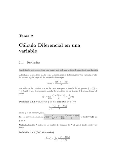
Tema 2<br />
<strong>Cálculo</strong> <strong>Difer<strong>en</strong>cial</strong> <strong>en</strong> <strong>una</strong><br />
<strong>variable</strong><br />
2.1. Derivadas<br />
La derivada nos proporciona <strong>una</strong> manera de calcular la tasa de cambio de <strong>una</strong> función<br />
Calculamos la velocidad media como la razón <strong>en</strong>tre la distancia recorrida <strong>en</strong> un intervalo<br />
de tiempo h y la longitud del intervalo de tiempo.<br />
vmedia =<br />
x(t + h) − x(t)<br />
,<br />
h<br />
este valor es la p<strong>en</strong>di<strong>en</strong>te m de la recta que pasa a través de los puntos (t, x(t)) y<br />
(t + h, x(t + h)). Si queremos calcular la velocidad <strong>en</strong> un tiempo t debemos tomar el<br />
límite<br />
x(t + h) − x(t)<br />
v(t) = lím<br />
=<br />
h→0 h<br />
d<br />
dt x(t)<br />
Definición 2.1.1 Una función f se dice derivable <strong>en</strong> x ⇐⇒<br />
f(x + h) − f(x)<br />
lím<br />
h→0 h<br />
existe y es un número finito.<br />
Si f es derivable, <strong>en</strong>tonces f ′ (x) = d<br />
f(x + h) − f(x)<br />
f(x) = lím<br />
dx h→0 h<br />
f <strong>en</strong> x.<br />
es la derivada de<br />
Nota. La función f ′ existe <strong>en</strong> los puntos del dominio de f tal que el límite existe y es<br />
finito.<br />
Definición 2.1.2 (Def. alternativa)<br />
f ′ (x0) = lím<br />
x→x0<br />
f(x) − f(x0)<br />
x − x0
2 <strong>Cálculo</strong> <strong>Difer<strong>en</strong>cial</strong> <strong>en</strong> <strong>una</strong> <strong>variable</strong><br />
Recta tang<strong>en</strong>te<br />
La recta que pasa por (x0, f(x0)) con p<strong>en</strong>di<strong>en</strong>te m = f ′ (x0) es la recta tang<strong>en</strong>te a f(x)<br />
<strong>en</strong> x0: y = m(x − x0) + f(x0).<br />
Propiedades<br />
1. (c1f + c2g) ′ = c1f ′ + c2g ′ , c1, c2 ∈ R.<br />
2. (f · g) ′ = f ′ g + fg ′<br />
3.<br />
<br />
f<br />
′<br />
=<br />
g<br />
f ′ g − fg ′<br />
g2 Teorema 2.1.3 (Regla de la Cad<strong>en</strong>a) Si g es derivable <strong>en</strong> x y f lo es <strong>en</strong> g(x),<br />
<strong>en</strong>tonces la función compuesta f ◦ g es derivable <strong>en</strong> x, y verifica<br />
(f ◦ g) ′ (x) = f ′ (g(x))g ′ (x)<br />
Nota. Con la regla de la cad<strong>en</strong>a podemos demostrar que<br />
(f −1 ) ′ (x) =<br />
1<br />
f ′ (f −1 (x)) .<br />
Podemos utilizar esta id<strong>en</strong>tidad para calcular las derivadas (arctan x) ′ y (ln x) ′ .<br />
Derivadas básicas<br />
1. c ′ = 0<br />
2. (x n ) ′ = nx n−1<br />
3. (e x ) ′ = e x , (log x) ′ = 1<br />
x<br />
4. (s<strong>en</strong> x) ′ = cos x, (cos x) ′ = −s<strong>en</strong> x, (tan x) ′ = 1<br />
cos 2 x<br />
5. (arctan x) ′ = 1<br />
1 + x 2 , (arcs<strong>en</strong> x)′ =<br />
6. (x) ′ = cosh, (cosh x) ′ = s<strong>en</strong>h x<br />
Teorema 2.1.4<br />
1<br />
√ 1 − x 2<br />
f derivable ⇒ f continua<br />
Teorema 2.1.5 (Teorema de Rolle) Sea f be derivable <strong>en</strong> (a, b) y continua <strong>en</strong> [a, b].<br />
Si f(a) = f(b), <strong>en</strong>tonces existe al m<strong>en</strong>os un número c ∈ (a, b) tal que<br />
f ′ (c) = 0.
2.1. Derivadas 3<br />
Teorema 2.1.6 (Teorema del Valor Medio) Sea f be derivable <strong>en</strong> (a, b) y continua<br />
<strong>en</strong> [a, b], <strong>en</strong>tonces existe al m<strong>en</strong>os un número c ∈ (a, b) tal que<br />
f ′ (c) =<br />
o, equival<strong>en</strong>tem<strong>en</strong>te f(b) − f(a) = f ′ (c)(b − a).<br />
f(b) − f(a)<br />
,<br />
b − a<br />
Teorema 2.1.7 (Regla de L’Hôpital) Sean f y g funciones derivables <strong>en</strong> (a, b), ex-<br />
f(x)<br />
0<br />
cepto posiblem<strong>en</strong>te <strong>en</strong> el punto x0 ∈ (a, b). Si lím es la indeterminación , <strong>en</strong>-<br />
x→x0 g(x) 0<br />
tonces<br />
f(x) f<br />
lím = lím<br />
x→x0 g(x) x→x0<br />
′ (x)<br />
g ′ (x) ,<br />
f<br />
siempre que lím<br />
x→x0<br />
′ (x)<br />
g ′ exista o sea infinito.<br />
(x)<br />
Ext<strong>en</strong>siones<br />
La regla de L’Hôpital se puede aplicar <strong>en</strong> los casos sigui<strong>en</strong>tes:<br />
Si la indeterminación es ∞<br />
∞<br />
Si el límite es x0 → ±∞<br />
A los límites laterales<br />
con todos los signos posibles.<br />
Derivación implícita<br />
Si la ecuación vi<strong>en</strong>e dada de manera implícita, F (x, y) = 0, hay que derivarla respecto<br />
a x y a partir de ahí obt<strong>en</strong>er dy<br />
dx .<br />
Derivadas de ord<strong>en</strong> superior<br />
Podemos hallar la derivada de <strong>una</strong> derivada:<br />
d 2 f<br />
dx 2 = f ′′ (x),<br />
d 3 f<br />
dx 3 = f ′′′ (x), · · · , dn f<br />
dx n = f (n) (x)
4 <strong>Cálculo</strong> <strong>Difer<strong>en</strong>cial</strong> <strong>en</strong> <strong>una</strong> <strong>variable</strong><br />
2.2. Extremos<br />
Definición 2.2.1 Sea f <strong>una</strong> función definida <strong>en</strong> un intervalo I:<br />
f(xm) es el mínimo global (o absoluto) de f <strong>en</strong> I si f(xm) ≤ f(x), ∀x ∈ I<br />
f(xM) es el máximo global (o absoluto) de f <strong>en</strong> I si f(xM) ≥ f(x), ∀x ∈ I<br />
Nota. Recordemos que si f es continua, <strong>en</strong> un intervalo cerrado y acotado [a, b], la<br />
función siempre alcanza su máximo y mínimo global .<br />
Definición 2.2.2 Sea f <strong>una</strong> función definida <strong>en</strong> un intervalo I, si t<strong>en</strong>emos un intervalo<br />
abierto I1 cont<strong>en</strong>i<strong>en</strong>do a x0<br />
f(x0) es un mínimo local de f <strong>en</strong> I si f(x0) ≤ f(x), ∀x ∈ I1<br />
f(x0) es un máximo local (o relativo) de f <strong>en</strong> I si f(x0) ≥ f(x), ∀x ∈ I1<br />
Definición 2.2.3 Sea f <strong>una</strong> función definida <strong>en</strong> x0. f ti<strong>en</strong>e un punto crítico <strong>en</strong> x0<br />
si<br />
f ′ (x0) = 0 o f ′ (x0) no existe<br />
Teorema 2.2.4 Si f ti<strong>en</strong>e un máximo o mínimo local <strong>en</strong> x0, <strong>en</strong>tonces x0 es un punto<br />
crítico de f.<br />
<strong>Cálculo</strong> de extremos globales de <strong>una</strong> función <strong>en</strong> un intervalo cerrado [a, b]<br />
1. Halla los puntos críticos de f <strong>en</strong> (a, b): f ′ (x0) = 0 o f ′ (x0) no exista<br />
2. Evalúa f <strong>en</strong> cada punto crítico de (a, b)<br />
3. Evalúa f <strong>en</strong> los extremos del intervalo: f(a) y f(b)<br />
4. El m<strong>en</strong>or valor es el mínimo global y el mayor, el máximo global<br />
Definición 2.2.5<br />
f es <strong>una</strong> función creci<strong>en</strong>te <strong>en</strong> un intervalo I si ∀x1, x2 ∈ I con x1 < x2 t<strong>en</strong>emos<br />
que f(x1) < f(x2).<br />
f es <strong>una</strong> función decreci<strong>en</strong>te <strong>en</strong> un intervalo I si ∀x1, x2 ∈ I con x1 < x2<br />
t<strong>en</strong>emos que f(x1) > f(x2).<br />
Teorema 2.2.6 Sea f <strong>una</strong> función continua <strong>en</strong> un intervalo cerrado [a, b] y derivable<br />
<strong>en</strong> (a, b)<br />
1. Si f ′ (x) > 0, ∀x ∈ (a, b) <strong>en</strong>tonces f es creci<strong>en</strong>te <strong>en</strong> [a, b].<br />
2. Si f ′ (x) < 0, ∀x ∈ (a, b) <strong>en</strong>tonces f es decreci<strong>en</strong>te <strong>en</strong> [a, b].<br />
3. Si f ′ (x) = 0, ∀x ∈ (a, b) <strong>en</strong>tonces f es constante <strong>en</strong> [a, b].
2.2. Extremos 5<br />
f ′ (x)<br />
Criterio de la primera derivada<br />
x < x0 x > x0 x0 (punto crítico)<br />
− + mínimo local<br />
+ − máximo local<br />
− − no extremo local<br />
+ + no extremo local<br />
Definición 2.2.7 Sea f derivable <strong>en</strong> un intervalo abierto I. La gráfica de f es<br />
convexa (cóncava hacia arriba) <strong>en</strong> I si f ′ es creci<strong>en</strong>te.<br />
cóncava (cóncava hacia abajo) <strong>en</strong> I si f ′ es decreci<strong>en</strong>te.<br />
Teorema 2.2.8 Sea f <strong>una</strong> función derivable dos veces <strong>en</strong> un intervalo abierto I<br />
Si f ′′ (x) > 0, ∀x ∈ I, <strong>en</strong>tonces la gráfica de f es convexa <strong>en</strong> I.<br />
Si f ′′ (x) < 0, ∀x ∈ I, <strong>en</strong>tonces la gráfica de f es cóncava <strong>en</strong> I.<br />
Definición 2.2.9 Sea f <strong>una</strong> función continua <strong>en</strong> un intervalo abierto I y sea x0 ∈ I.<br />
f ti<strong>en</strong>e un punto de inflexión <strong>en</strong> x0 si la concavidad cambia <strong>en</strong> x0 (convexa ↔<br />
cóncava).<br />
Teorema 2.2.10 Si x0 es un punto de inflexión de f, <strong>en</strong>tonces f ′′ (x0) = 0 o f ′′ (x0)<br />
no existe.<br />
Teorema 2.2.11 Sea f <strong>una</strong> función tal que f ′ (x0) = 0 y derivable dos veces <strong>en</strong> un<br />
intervalo abierto cont<strong>en</strong>i<strong>en</strong>do a x0<br />
si f ′′ (x0) > 0, <strong>en</strong>tonces f ti<strong>en</strong>e un mínimo local <strong>en</strong> x0.<br />
si f ′′ (x0) < 0, <strong>en</strong>tonces f ti<strong>en</strong>e un máximo local <strong>en</strong> x0.<br />
Si f ′′ (x0) = 0 el criterio no funciona, puede ser cualquier cosa.<br />
f ′ (x0) f ′′ (x0) gráfica<br />
+ − creci<strong>en</strong>te, cóncava<br />
− − decreci<strong>en</strong>te, cóncava<br />
+ + creci<strong>en</strong>te, convexa<br />
− + decreci<strong>en</strong>te, convexa<br />
0 + mínimo local<br />
0 − máximo local<br />
0 0 ?
6 <strong>Cálculo</strong> <strong>Difer<strong>en</strong>cial</strong> <strong>en</strong> <strong>una</strong> <strong>variable</strong><br />
2.3. Gráficas<br />
1. Dominio<br />
2. Intersección con el eje x → f(x) = 0<br />
Intersección con el eje y → f(0) = y<br />
3. Simetrías<br />
f(−x) = +f(x) → par<br />
f(−x) = −f(x) → impar<br />
Periodicidad → f(x + T ) = f(x)<br />
4. Asíntotas:<br />
Vertical → lím f(x) = ±∞<br />
x→x0<br />
Horizontal → lím f(x) = H<br />
x→±∞<br />
Oblicua → lím f(x) − (mx + b) = 0 → m = lím<br />
x→±∞ x→∞<br />
5. Continuidad: lím f(x) = f(x0)<br />
x→x0<br />
6. Derivada: monotonía y puntos críticos<br />
f ′ (x) > 0→ creci<strong>en</strong>te<br />
f ′ (x) < 0 → decreci<strong>en</strong>te<br />
f ′ (x) = 0 o f ′ (x) no exista → puntos críticos<br />
7. Máximos y mínimos locales: x0 → punto crítico<br />
8. Concavidad<br />
f ′ (x0) = 0, f ′′ (x0) > 0 → mínimo local<br />
f ′ (x0) = 0, f ′′ (x0) < 0 → máximo local<br />
f ′ (x) : − ↦→ + → mínimo local<br />
f ′ (x) : + ↦→ − → máximo local<br />
f ′′ (x) > 0 → convexa<br />
f ′′ (x) < 0 → cóncava<br />
9. Puntos de inflexión. La concavidad cambia. f ′′ (x0) = 0 o ∄f ′′ (x0)<br />
10. Máximos y mínimos globales<br />
f(x)<br />
, b = lím (f(x) − mx)<br />
x x→∞
2.4. Polinomio de Taylor 7<br />
2.4. Polinomio de Taylor<br />
La idea es aproximar <strong>una</strong> función f(x) por un polinomio P (x). El polinomio de<br />
Taylor es el polinomio que mejor aproxima a <strong>una</strong> función <strong>en</strong> un punto x0<br />
<br />
<strong>una</strong> constante → P (x) = f(x0)<br />
Si aproximamos f(x) por<br />
<strong>una</strong> recta → P (x) = f(x0) + f ′ (x0)(x − x0)<br />
Definición 2.4.1 Si f es derivable n veces <strong>en</strong> x0, <strong>en</strong>tonces el polinomio<br />
Pn(x) = f(x0) + f ′ (x0)(x − x0) + f ′′ (x0)<br />
2!<br />
es el polinomio de Taylor de grado n de f c<strong>en</strong>trado <strong>en</strong> x0.<br />
(x − x0) 2 + · · · f (n) (x0)<br />
(x − x0)<br />
n!<br />
n<br />
Nota. Para x0 = 0 el polinomio también se llama Polinomio de Mac Laurin.<br />
ERROR<br />
El polinomio es <strong>una</strong> aproximación de f(x), por lo que se comete un error<br />
|Rn(x)| = |f(x) − P (x)|. Exist<strong>en</strong> muchas fórmulas para este error, pero la idea es que<br />
todas ellas verifican<br />
f(x) − Pn(x)<br />
lím<br />
x→x0 (x − x0) n = 0.<br />
→ Rn(x) = o (x − x0) n . Notación: f(x) = o g(x) cuando x → x0 ⇐⇒<br />
lím<br />
x→x0<br />
f(x)<br />
= 0.<br />
g(x)<br />
En el sigui<strong>en</strong>te teorema t<strong>en</strong>emos <strong>una</strong> fórmula para el error |Rn(x)|:<br />
Teorema 2.4.2 Sea f(x) <strong>una</strong> función derivable n + 1 veces <strong>en</strong> un intervalo abierto I,<br />
<strong>en</strong>tonces ∀x0, x ∈ I t<strong>en</strong>emos que<br />
f(x) = Pn(x) + Rn(x) = f(x0) + f ′ (x0)(x − x0) + · · · f (n) (x0)<br />
n!<br />
(x − x0) n + Rn(x),<br />
Rn(x) = f (n+1) (ξ)<br />
(n + 1)! (x − x0) (n+1) , ξ es un punto <strong>en</strong> el intervalo abierto definido por x0 y x.