Presentación de Javier Escobal - Grade

Desigualdad espacial en el Perú en las
últimas tres décadas
Javier Escobal
Carmen Ponce

Esquema de la Presentación
o Percepciones sobre la evolución de la Desigualdad
o Necesidad de construir indicadores de Pobreza y
Desigualdad consistentes para antes del 2004.
• Aplicación de la metodología sugerida por Elbers, Lanjouw y
Lanjouw (2004)
o Estimación del gasto per-cápita, pobreza y medidas de
desigualdad a mayores niveles de desagregación
geográfica
o El problema de la cola de la distribución: corrección de las
medidas de desigualdad por sub-reporte del segmento más
rico
o
o
Polarización espacial
Explicación preliminar sobre las tendencias identificadas:
o Elasticidades crecimiento pobreza

Percepciones
o
o
“Mientras que la desigualdad obtenida a partir de las
encuestas se reduce, la obtenida a partir de las cuentas
nacionales se incrementa”. (Otra Mirada: Informe N°255,
09/06/2010)
“...si tomamos en cuenta el crecimiento exponencial de
las utilidades mineras en los últimos años, resulta válida
la hipótesis que la desigualdad en el ingreso se haya
incrementado”. (Otra Mirada: Informe N°294,
12/08/2010)

Problemas de comparabilidad intertemporal
Figueroa 50s, 60s CEPAL 1995‐2005 diferencia
Argentina 0.43 0.48 0.05
Brazil 0.58 0.56 ‐0.02
Chile 0.50 0.55 0.05
Colombia 0.58 0.55 ‐0.03
Costa Rica 0.37 0.47 0.10
Mexico 0.54 0.51 ‐0.03
Peru 0.62 0.50 ‐0.12
EEUU 0.36 0.40 0.04
Fuentes: Figueroa, A. y R. Weisskoff (1974): “Visión de las
Pirámides Sociales: Distribución del ingreso en America Latina”.
PUCP Documentos de Trabajo. No. 15.
PNUD (2010): Informe Regional sobre Desarrollo Humano para
América Latina y el Caribe 2010: Actuar sobre el futuro: romper la
transmisión intergeneracional de la desigualdad

Necesidad de construir indicadores de Pobreza
y Desigualdad consistentes para antes del 2004
o
o
o
o
A partir del 2004 (datos anuales) o 2002-IV trimestre, la
información de las encuestas de hogares son consistentes. Para
antes de esa fecha la data no es comparable.
Las encuestas de hogares no son compatibles con cuentas
nacionales (subestiman el gasto de consumo). Esto estaría
asociado a sub-reporte de los más ricos.
Los niveles de inferencia de los datos de pobreza y de la
distribución del ingreso no son suficientemente detallados como
para darnos una idea de la distribución a niveles de
desagregación espacial mayor (i.e. Provincias)
Es posible enfrentar el problema combinando la información de
encuestas, la información del censo de población y otra
información complementaria (censo agrario, Censo continuo,
registros administrativos. Información geográfica, etc.

Combinando encuestas de hogares y Censos
o Metodología desarrollada por Elbers, Lanjouw y Lanjouw (2004)
o La relación funcional a estimar en la primera etapa tiene la siguiente
forma:
o
G = x ' β +
ch
ch
G ch
es el logaritmo del gasto per cápita del hogar h, residente del distrito
c, X ch
es el vector de características del hogar h (incluye características
individuales y distritales del hogar h), y β es el vector de parámetros a
estimar.
u
ch
o
o
Un elemento central en esta metodología es la modelación del error. El
vector u h
(que se asume satisface el supuesto E[ u y se distribuye
h| x
h]=0
como u ≈ f (0, ) ) tiene la siguiente forma:
∑
u
ch
=η + ε
c
ch
Donde η c
es el componente “espacial” del error, común a los hogares que
residen en el distrito c, y ε ch
es el componente idiosincrásico del error.

Ajuste de requerimientos calóricos y
coeficiente de Engel
Se requiere
compatibilizar,
gastos, líneas de
pobreza, etc.
Requerimientos calóricos per cápita utilizados en el cálculo de la línea
Dominio
Requerimientos calóricos oficiales Requerimientos calóricos ajustados *
1985 1994 2006 1985 1994 2006
Costa Urbana (sin LM) 2,371 2,371 2,194 2,161 2,167 2,214
Costa Rural 2,371 2,371 2,194 2,133 2,131 2,218
Sierra Urbana 2,648 2,648 2,194 2,140 2,181 2,226
Sierra Rural 2,648 2,648 2,133 2,071 2,120 2,148
Selva Urbana 2,385 2,385 2,194 2,129 2,131 2,202
Selva Rural 2,385 2,385 2,133 2,091 2,088 2,162
Lima Metropolitana (LM) 2,371 2,371 2,232 2,185 2,220 2,229
Fuente: ENNIV 1985, ENNIV 1994, ENAHO 2006
Coeficientes de Engel utilizados en el cálculo de la línea
Dominio
Coeficiente de Engel oficiales Coeficiente de Engel ajustados *
1985 1994 2006 1985 1994 2006
Costa Urbana (sin LM) 56% 49% 51% 44% 44% 43%
Costa Rural 69% 54% 58% 54% 54% 55%
Sierra Urbana 58% 47% 52% 49% 42% 43%
Sierra Rural 78% 64% 64% 69% 67% 66%
Selva Urbana 50% 52% 60% 51% 50% 47%
Selva Rural 56% 60% 63% 65% 61% 63%
Lima Metropolitana (LM) 57% 50% 45% 42% 42% 41%
Urbano 44% 43% 42%
Rural 65% 63% 64%
Nacional 49% 47% 48%
Fuente: ENNIV 1985, ENNIV 1994, ENAHO 2006

Validación Interna: 1994
TASA DE POBREZA
ENNIV 1985 Estimación Censo 1981
Dominio
Tasa de Intervalo de Confianza Tasa de Error
Geográfico
Pobreza
(95%)
Pobreza Estándar
Costa Urbana 47% 40% 53% 50% 0.01
Costa Rural 52% 43% 62% 47% 0.01
Sierra Urbana 31% 22% 40% 33% 0.03
Sierra Rural 42% 37% 47% 40% 0.02
Selva Urbana 32% 13% 51% 26% 0.02
Selva Rural 58% 47% 69% 54% 0.03
Lima Metropolitana 28% 23% 32% 32% 0.01
Urbano 34% 30% 37% 37% 0.01
Rural 47% 42% 52% 43% 0.02
Nacional 39% 36% 42% 40% 0.01
Líneas de pobreza total calculada sobre poblaciones de referencia para cada dominio y engels por dominio.
Nota general a los tres cuadros: El Censo 1981 no incluye información de Loreto, San Martín y Apurímac,
lo que afecta el nivel de precisión de los indicadores de Selva Urbana fundamentalmente.

Validación Interna: 1994 y 2006
TASA DE POBREZA
ENNIV 1994 Estimación Censo 1993
Dominio
Tasa de Intervalo de Confianza Tasa de Error
Geográfico
Pobreza
(95%)
Pobreza Estándar
Costa Urbana 57% 50% 64% 59% 0.01
Costa Rural 65% 54% 76% 62% 0.01
Sierra Urbana 45% 37% 53% 49% 0.01
Sierra Rural 56% 50% 62% 57% 0.01
Selva Urbana 43% 36% 51% 42% 0.02
Selva Rural 67% 61% 73% 67% 0.01
Lima Metropolitana 49% 44% 54% 48% 0.03
Urbano 50% 47% 53% 51% 0.01
Rural 59% 55% 63% 60% 0.01
Nacional 53% 51% 56% 54% 0.01
Líneas de pobreza total calculada sobre poblaciones de referencia para cada dominio y engels por dominio.
TASA DE POBREZA
ENAHO 2006 Estimación Censo 2005
Dominio
Tasa de Intervalo de Confianza Tasa de Error
Geográfico
Pobreza
(95%)
Pobreza Estándar
Costa Urbana 44% 41% 47% 43% 0.02
Costa Rural 56% 50% 61% 55% 0.01
Sierra Urbana 56% 53% 59% 55% 0.01
Sierra Rural 76% 73% 78% 76% 0.01
Selva Urbana 66% 61% 71% 65% 0.02
Selva Rural 64% 61% 68% 63% 0.02
Lima Metropolitana 33% 30% 35% 31% 0.02
Urbano 43% 42% 45% 42% 0.01
Rural 70% 68% 72% 70% 0.01
Nacional 53% 51% 54% 51% 0.01
Líneas de pobreza total calculada sobre poblaciones de referencia para cada dominio y engels por dominio.

Estimaciones Alternativas de Pobreza
Dominio
Oficial * Ajustada **
1985 1994 2006 1985 1994 2006
Costa Urbana (sin LM) 42% 46% 30% 47% 57% 44%
Costa Rural 50% 55% 49% 52% 65% 56%
Sierra Urbana 35% 41% 40% 31% 45% 56%
Sierra Rural 49% 59% 76% 42% 56% 76%
Selva Urbana 48% 36% 50% 32% 43% 66%
Selva Rural 69% 60% 62% 58% 67% 64%
Lima Metropolitana (LM) 26% 38% 24% 28% 49% 33%
Urbano 33% 40% 31% 34% 50% 43%
Rural 54% 59% 69% 47% 59% 70%
Nacional 41% 47% 44% 39% 53% 53%
Fuente: ENNIV 1985, ENNIV 1994, ENAHO 2006
Tasa de Pobreza
Las cifras “oficiales” tienen problemas de
comparabilidad y pueden mostrar tendencias erróneas

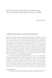
Crecimiento Provincial 1993 - 2005
Crecimiento del gpc 93-05
CRECIM9305
-0.407762 - -0.154864
-0.154863 - 0.010994
0.010995 - 0.233164
0.233165 - 0.498624
0.498625 - 0.948419

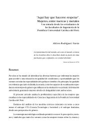
Cambios en la Pobreza Provincial 1993 - 2005
cambio en tasa de pobreza 93-05
-0.319444 - -0.104479
-0.104478 - 0.021221
0.021222 - 0.108782
0.108783 - 0.190185
0.190186 - 0.316572

Dinámicas de Pobreza 1981 – 1993 - 2005
1981 1993 2005
provincia 2005
0.167795 - 0.300000
0.300001 - 0.450000
0.450001 - 0.600000
0.600001 - 0.750000
0.750001 - 0.900000

Concentración espacial de dinámicas
1993 2005

Evolución de la Desigualdad
○ Luego de compatibilizar los gastos entre encuestas y ajustar
el gasto usando deflactores espaciales:
Evolución de la Desigualdad (Gini)
1985 1994 2006
Urbano 0.42 0.37 0.36
Rural 0.40 0.37 0.30
Peru 0.45 0.41 0.40
Desigualdad en el acceso a la educación *
(Años de educación del Jefe del hogar)
1981 1993 2007
Theil 0.249 0.216 0.146
Gini 0.365 0.350 0.256
Descomposición (importancia del componente entre grupos)
Grupos 1981 1993 2007
rural/urbano 29.76% 16.69% 33.52%
jerarquía urbana 10.06% 8.31% 14.88%
* Se excluye a Apurímac, Loreto y San Martín.

ENAHO versus Cuentas Nacionales
○ Incompatibilidad de las Encuestas de Hogares con Cuentas
Nacionales
▪
▪
▪
▪
“Las Encuestas de Hogares no registran los ingresos (gastos) de los más
ricos
Esto se refleja en el hecho que el gasto de consumo registrado en
Cuentas Nacionales es muy superior al gasto per cápita de ENAHO
(aprox. 70% más alto!)
Yamada y Castro (2006) muestran que cuando se ajusta el gini por
cuentas nacionales - usando la corrección sugerida por Lopez y Serven
(2006) el indicador se incrementa sustantivamente (de 0.376 a 0.566 en
el 2004)
Si uno ajusta los Gini que hemos calculado, los indicadores,
como era de esperar, aumentan PERO la tendencia es muy
parecida

Evolución de la Desigualdad ... incluyendo
corrección cuentas nacionales
○ Si se presume que la distribución del ingreso (gasto per cápita)
es log-normal
Gini ‐ Corrección por Cuentas Nacionales
1985 1994 2004 2006 2009
Gini ‐ Original 0.45 0.41 0.37 0.39 0.36
Gini ‐ Corregido 0.52 0.52 0.55 0.54 0.50
○ Los resultados parecen ser similares si se reemplaza el supuesto
de log-normalidad y se ajusta la distribución a una del tipo
Singh-Maddala o Dagum (u otra que tenga colas más anchas)
○ A nivel agregado no habría evidencia de incremento del gini.
○ Sin embargo, esto no significa que la desigualdad no se esté
incrementando en alguna dimensión relevante (urbano/rural,
más educado / menos educado, etc.)

Cambios en desigualdad 1993-2005
Descomposición de la Desigualdad del Gasto per‐cápita
(a partir del Theil del Gasto Per‐capita real a precios de Lima)
Entre Categorias Entre Categorias
Grupos
1993
2005
rural/urbano 1.3% 10.4%
nivel educativo 13.2% 26.2%
rural/urbano+ Educ 13.4% 27.9%
provincias 4.9% 20.7%
rural/urbano+provincias 7.0% 22.3%
electricidad 5.0% 12.3%
rural/urbano+ Electricidad 5.3% 14.7%
jerarquía urbana 1.5% 13.1%
Theil 0.232 0.223
No pasa
mucho
en el
agregado
pero las
diferenci
as entre
grupos
se
amplían!

Cambios en desigualdad 1981-1993-2005
Descomposición de la Desigualdad del Gasto per‐cápita
(a partir del Theil del Gasto Per‐capita real a precios de Lima)
Entre Categorias Entre Categorias Entre Categorias
Grupos
1981
1993
2005
rural/urbano 0.4% 1.1% 10.7%
nivel educativo 10.5% 13.4% 26.3%
rural/urbano+ Educ 11.3% 13.7% 28.2%
provincias 7.3% 5.5% 20.2%
rural/urbano+provincias 9.8% 7.1% 21.7%
electricidad 3.7% 5.1% 12.1%
rural/urbano+ Electricidad 4.7% 5.6% 14.6%
jerarquía urbana 0.7% 1.4% 13.6%
Theil 0.306 0.233 0.223
* Se excluye a Apurímac, Loreto y San Martín.

Reducción de la desigualdad al interior de las distintas
jerarquías urbano-rurales (en un contexto de creciente
polarización espacial
Theil del Gasto Per‐capita real a precios de Lima
Grupos
Intra‐categorías
1993
Intra‐categorías
2005
Grandes ciudades 0.22 0.22
Ciudades Intermedias 0.24 0.18
Rurales 0.24 0.17
Theil del Gasto Per‐capita real a precios de Lima
Grupos
Intra‐categorías
1981
Intra‐categorías
1993
Intra‐categorías
2005
Grandes ciudades 0.28 0.22 0.21
Ciudades Intermedias 0.33 0.24 0.17
Rurales 0.33 0.23 0.17
* Se excluye a Apurímac, Loreto y San Martín.

Distribución espacial del Bienestar
Evolución del Gasto Per capita a precios de Lima (welfare ratio)
Grupos 1981 1993 2005
Grandes ciudades 2.075 1.550 1.840
Ciudades Intermedias 1.834 1.419 1.269
Rurales 1.931 1.348 1.046
Nacional 1.972 1.460 1.495
* Se excluye a Apurímac, Loreto y San Martín.
Cambios en la Distribución espacial del Gasto Per capita (a precios de Lima)
Grupos 1981 1993 2005
Grandes ciudades 43% 48% 50%
Ciudades Intermedias 21% 23% 24%
Rurales 36% 30% 27%
Nacional 100% 100% 100%
* Se excluye a Apurímac, Loreto y San Martín.

Dinámica de la Pobreza por tipo de provincia
1981, 1993 y 2005
Nota: No incluye a los departamentos de Apurímac, Loreto y San Martín. En el Anexo 8.1 se muestran los resultados de 1993 y 2005 que incluyen a estos departamentos. No hay diferencias
importantes en estos indicadores entre ambas tablas.
Fuente: Estimaciones propias en base a los censos de Población 1981, 1993 y 2005, las ENNIV 1985, 1994 y la ENAHO 2006.

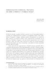
Cambios en la distribución del gasto a nivel
Provincial
(a) Nacional
(b) Distribución Provincial
0 .2 .4 .6 .8
Distribución del Gasto Per Cápita entre 1993 y 2005
-1 0 1 2 3
(welfare ratio deflacftado por líneas de de pobreza - escala logarítmica)
1993 2005
Cambios en la distribución del gasto per cápita entre 1993 y 2005
0
kdensity
1
lwrlpt93
2 3
-.5 0 .5 1
Welfare ratio deflactado por línea de pobreza
kdensity lwrlpt93
kdensity lwrlpt05
.2 .4 .6 .8 1 1.2
kdensity lwrlpt05
(c) Provincias con Ciudades Intermedias
(d) Provincias Rurales
Cambios en la distribución del gasto per cápita entre 1993 y 2005
.5 1
kdensity
1.5
lwrlpt93
2 2.5
0 .5 1 1.5 2 2.5
kdensity lwrlpt05
Cambios en la distribución del gasto per cápita entre 1993 y 2005
0
kdensity
1
lwrlpt93
2 3
0 .5 1 1.5 2
kdensity lwrlpt05
-.4 -.2 0 .2 .4 .6
Welfare ratio deflactado por línea de pobreza
kdensity lwrlpt93
kdensity lwrlpt05
-.5 0 .5 1
Welfare ratio deflactado por línea de pobreza
kdensity lwrlpt93
kdensity lwrlpt05

Explicación preliminar sobre las tendencias
identificadas: El reto de la desigualdad y el Perú rural
o
o
Desigualdad sigue alta y aunque en el agregado muestre cierta
tendencia decreciente hay ciertas dimensiones de desigualdad (en
particular la desigualdad espacial) que está creciendo
Esta desigualdad se origina
• Desigualdad de accesos a servicios (más allá de los básicos..)
• Desigualdad en el acceso a factores de producción
• Desigualdad en la posibilidad de ejercer derechos ciudadanos
→ Desigualdad de Oportunidades

Explicación preliminar sobre las tendencias
identificadas

Concentración espacial de la Pobreza

Gracias