Tablas de Probabilidades - ITAM
Tablas de Probabilidades - ITAM
Tablas de Probabilidades - ITAM

You also want an ePaper? Increase the reach of your titles
YUMPU automatically turns print PDFs into web optimized ePapers that Google loves.
<strong>Tablas</strong> <strong>de</strong> Probabilida<strong>de</strong>s 40<br />
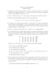
12. Distribución <strong>de</strong>l estadístico D <strong>de</strong> Kolmogorov-Smirnov<br />
Sea F ∗ la distribución conocida, F la distribución <strong>de</strong><br />
la variable X y F n la función <strong>de</strong> distribución empírica.<br />
Suponemos que X es una variable aleatoria continua.<br />
Para probar: H 0:F(x) = F ∗ (x)<br />
D = sup{|F ∗ (x) − F n(x)|}<br />
x<br />
Para probar: H 0:F(x) ≥ F ∗ (x)<br />
D + = sup{F ∗ (x) − F n(x)}<br />
x<br />
Para probar: H 0:F(x) ≤ F ∗ (x)<br />
p<br />
α<br />
0 x 1<br />
D − = sup{F n(x) − F ∗ (x)}<br />
x<br />
En los tres casos, la hipótesis nula <strong>de</strong>be rechazarse si el estadístico correspondiente es mayor que el cuantil al nivel<br />
<strong>de</strong> significancia <strong>de</strong>seado ∗ . Para n > 50 se presenta una aproximación <strong>de</strong>l cuantil correcto utilizando la distribución<br />
asintótica <strong>de</strong> los estadísticos ∗∗ .<br />
Tabla 12A. Valores críticos D + (α;n)<br />
<strong>de</strong> la distribución <strong>de</strong> Kolmogorov-Smirnov.<br />
p<br />
p<br />
0.99 0.975 0.95 0.90 0.99 0.975 0.95 0.90<br />
α<br />
α<br />
n 0.01 0.025 0.05 0.010 n 0.01 0.025 0.05 0.10<br />
1 0.990 0.975 0.950 0.900 26 0.290 0.259 0.233 0.204<br />
2 0.900 0.842 0.776 0.684 27 0.284 0.254 0.229 0.200<br />
3 0.785 0.708 0.636 0.565 28 0.279 0.250 0.225 0.197<br />
4 0.689 0.624 0.565 0.493 29 0.275 0.246 0.221 0.193<br />
5 0.627 0.563 0.509 0.447 30 0.270 0.242 0.218 0.190<br />
6 0.577 0.519 0.468 0.410 31 0.266 0.238 0.214 0.187<br />
7 0.538 0.483 0.436 0.382 32 0.262 0.234 0.211 0.184<br />
8 0.507 0.454 0.410 0.358 33 0.258 0.231 0.208 0.182<br />
9 0.480 0.430 0.387 0.339 34 0.254 0.227 0.205 0.179<br />
10 0.457 0.409 0.369 0.323 35 0.251 0.224 0.202 0.177<br />
11 0.437 0.391 0.352 0.308 36 0.247 0.221 0.199 0.174<br />
12 0.419 0.375 0.338 0.296 37 0.244 0.218 0.196 0.172<br />
13 0.404 0.361 0.326 0.285 38 0.241 0.215 0.194 0.170<br />
14 0.390 0.349 0.314 0.275 39 0.238 0.213 0.191 0.168<br />
15 0.377 0.338 0.304 0.266 40 0.235 0.210 0.189 0.165<br />
16 0.366 0.327 0.295 0.258 41 0.232 0.208 0.187 0.163<br />
17 0.355 0.318 0.286 0.250 42 0.229 0.205 0.185 0.162<br />
18 0.346 0.309 0.279 0.244 43 0.227 0.203 0.183 0.160<br />
19 0.337 0.301 0.271 0.237 44 0.224 0.201 0.181 0.158<br />
20 0.329 0.294 0.265 0.232 45 0.222 0.198 0.179 0.156<br />
21 0.321 0.287 0.259 0.226 46 0.219 0.196 0.177 0.155<br />
22 0.314 0.281 0.253 0.221 47 0.217 0.194 0.175 0.153<br />
23 0.307 0.275 0.247 0.216 48 0.215 0.192 0.173 0.151<br />
24 0.301 0.269 0.242 0.212 49 0.213 0.190 0.171 0.150<br />
25 0.295 0.264 0.238 0.208 50 0.211 0.188 0.170 0.148<br />
n > 50<br />
1.517<br />
√ n<br />
1.358<br />
√ n<br />
1.224<br />
√ n<br />
1.073<br />
√ n<br />
∗ Nota: La distribución <strong>de</strong>l estadístico D − es la misma que la <strong>de</strong> D + . Los valores críticos para el estadístico D son los<br />
presentados para el nivel 2α.<br />
∗∗ Nota: El error <strong>de</strong> aproximación es menor que 4 × 10 −3 para ambas pruebas.<br />
c○ E. Barrios y J. A. García<br />
v.1.05