Les mod`eles de Black & Scholes et Merton : Analyse de leurs ...
Les mod`eles de Black & Scholes et Merton : Analyse de leurs ...
Les mod`eles de Black & Scholes et Merton : Analyse de leurs ...

You also want an ePaper? Increase the reach of your titles
YUMPU automatically turns print PDFs into web optimized ePapers that Google loves.
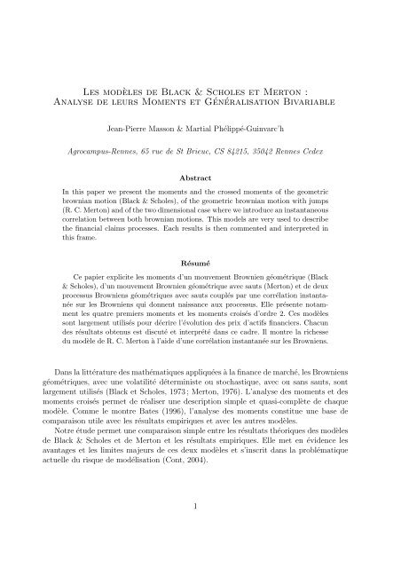
<strong>Les</strong> modèles <strong>de</strong> <strong>Black</strong> & <strong>Scholes</strong> <strong>et</strong> <strong>Merton</strong> :<br />
<strong>Analyse</strong> <strong>de</strong> <strong>leurs</strong> Moments <strong>et</strong> Généralisation Bivariable<br />
Jean-Pierre Masson & Martial Phélippé-Guinvarc’h<br />
Agrocampus-Rennes, 65 rue <strong>de</strong> St Brieuc, CS 84215, 35042 Rennes Ce<strong>de</strong>x<br />
Abstract<br />
In this paper we present the moments and the crossed moments of the geom<strong>et</strong>ric<br />
brownian motion (<strong>Black</strong> & <strong>Scholes</strong>), of the geom<strong>et</strong>ric brownian motion with jumps<br />
(R. C. <strong>Merton</strong>) and of the two dimensional case where we introduce an instantaneous<br />
correlation b<strong>et</strong>ween both brownian motions. This mo<strong>de</strong>ls are very used to <strong>de</strong>scribe<br />
the financial claims processes. Each results is then commented and interpr<strong>et</strong>ed in<br />
this frame.<br />
Résumé<br />
Ce papier explicite les moments d’un mouvement Brownien géométrique (<strong>Black</strong><br />
& <strong>Scholes</strong>), d’un mouvement Brownien géométrique avec sauts (<strong>Merton</strong>) <strong>et</strong> <strong>de</strong> <strong>de</strong>ux<br />
processus Browniens géométriques avec sauts couplés par une corrélation instantanée<br />
sur les Browniens qui donnent naissance aux processus. Elle présente notamment<br />
les quatre premiers moments <strong>et</strong> les moments croisés d’ordre 2. Ces modèles<br />
sont largement utilisés pour décrire l’évolution <strong>de</strong>s prix d’actifs financiers. Chacun<br />
<strong>de</strong>s résultats obtenus est discuté <strong>et</strong> interprété dans ce cadre. Il montre la richesse<br />
du modèle <strong>de</strong> R. C. <strong>Merton</strong> à l’ai<strong>de</strong> d’une corrélation instantanée sur les Browniens.<br />
Dans la littérature <strong>de</strong>s mathématiques appliquées à la finance <strong>de</strong> marché, les Browniens<br />
géométriques, avec une volatilité déterministe ou stochastique, avec ou sans sauts, sont<br />
largement utilisés (<strong>Black</strong> <strong>et</strong> <strong>Scholes</strong>, 1973 ; <strong>Merton</strong>, 1976). L’analyse <strong>de</strong>s moments <strong>et</strong> <strong>de</strong>s<br />
moments croisés perm<strong>et</strong> <strong>de</strong> réaliser une <strong>de</strong>scription simple <strong>et</strong> quasi-complète <strong>de</strong> chaque<br />
modèle. Comme le montre Bates (1996), l’analyse <strong>de</strong>s moments constitue une base <strong>de</strong><br />
comparaison utile avec les résultats empiriques <strong>et</strong> avec les autres modèles.<br />
Notre étu<strong>de</strong> perm<strong>et</strong> une comparaison simple entre les résultats théoriques <strong>de</strong>s modèles<br />
<strong>de</strong> <strong>Black</strong> & <strong>Scholes</strong> <strong>et</strong> <strong>de</strong> <strong>Merton</strong> <strong>et</strong> les résultats empiriques. Elle m<strong>et</strong> en évi<strong>de</strong>nce les<br />
avantages <strong>et</strong> les limites majeurs <strong>de</strong> ces <strong>de</strong>ux modèles <strong>et</strong> s’inscrit dans la problématique<br />
actuelle du risque <strong>de</strong> modélisation (Cont, 2004).<br />
1
1 <strong>Les</strong> modèles<br />
L’ Équation Différentielle Stochastique du modèle <strong>de</strong> <strong>Black</strong> & <strong>Scholes</strong> est :<br />
dFt = (µF − λF .k (1)<br />
F ).Ft.dt + σF .Ft.dW F<br />
t<br />
où Ft est le prix à l’instant t ∈ [0, +∞). 1 µF est le paramètre constant (appelé aussi dérive).<br />
σF est le paramètre <strong>de</strong> volatilité. W F<br />
t est un mouvement Brownien standard. L’ Équation<br />
Différentielle Stochastique du modèle <strong>de</strong> R. C. <strong>Merton</strong> est :<br />
dFt = (µF − λF .kF ).Ft.dt + σF .Ft.dW F<br />
t + (S F − 1).Ft.dπ F<br />
où nous avons en sus : λF l’intensité du processus <strong>de</strong> Poisson π F <strong>de</strong>s sauts S F , <strong>et</strong> kF =<br />
E[S F − 1].<br />
On notera N F t le nombre aléatoire <strong>de</strong> sauts sur Ft entre 0 <strong>et</strong> t. En l’absence <strong>de</strong>s<br />
2 <strong>de</strong>rniers termes <strong>de</strong> l’équation 2, la dynamique est déterministe <strong>et</strong> exponentielle. En<br />
l’absence du <strong>de</strong>rnier terme la dynamique est stochastique <strong>et</strong> le processus est le Brownien<br />
géométrique du modèle <strong>de</strong> <strong>Black</strong> & <strong>Scholes</strong>. Dans le modèle compl<strong>et</strong> le <strong>de</strong>rnier terme<br />
décrit le saut additif. <strong>Les</strong> instants <strong>de</strong> saut sont gouvernés par le processus Poissonnien <strong>de</strong><br />
paramètre λF . La fonction d’impulsion S F − 1 produit un saut fini sur F (<strong>de</strong> F à S F .F )<br />
<strong>et</strong> le saut, aléatoire par S F <strong>et</strong> F , est égal à (S F − 1).F .<br />
Précisons le choix <strong>de</strong> modélisation fait par R. C. <strong>Merton</strong> ; le processus <strong>de</strong> saut est centré<br />
sur sa moyenne. Le processus S F − 1 .dπ F − λF .kF .dt est centré ; c’est une martingale<br />
purement discontinue à variation finie. Nous supposons que les variables aléatoires S F sont<br />
indépendantes <strong>et</strong> i<strong>de</strong>ntiquement distribuées <strong>de</strong> distribution log-normale <strong>de</strong> paramètres mF<br />
<strong>et</strong> v 2 F (ln SF ∼ N (mF , v 2 F )). L’espérance <strong>et</strong> la variance <strong>de</strong>s sauts SF sont respectivement<br />
égales à kF + 1 <strong>et</strong> τ 2 <br />
où : kF + 1 = exp mF + v2 <br />
F <strong>et</strong> τ 2<br />
2 = (kF + 1) 2 . [exp(v2 F ) − 1] .<br />
La résolution <strong>de</strong> l’ Équation Différentielle Stochastique du modèle <strong>de</strong> R. C. <strong>Merton</strong><br />
donne :<br />
<br />
Ft = F0. exp µF − λF .kF − 1<br />
2 σ2 <br />
F .t + σF .W F<br />
<br />
t .<br />
N F t<br />
S F j<br />
Nous en déduisons simplement la résolution <strong>de</strong> l’ Équation Différentielle Stochastique du<br />
modèle <strong>de</strong> <strong>Black</strong> & <strong>Scholes</strong> (λ = 0) :<br />
<br />
Ft = F0. exp µF − 1<br />
2 σ2 <br />
F .t + σF .W F<br />
<br />
t<br />
1 Nous ajoutons dores <strong>et</strong> déjà l’indice F à chaque paramètre <strong>de</strong> Ft en vu <strong>de</strong> la généralisation multidi-<br />
mensionnelle <strong>de</strong> l’analyse <strong>de</strong>s moments.<br />
2<br />
j=1<br />
(1)<br />
(2)<br />
(3)<br />
(4)
Nous noterons kF = k (1)<br />
F ≡ E[SF −1] ; puis k (2)<br />
S F<br />
F ≡ E<br />
<br />
2<br />
− 1 , . . . , k (n)<br />
F ≡ E SF n <br />
− 1 .<br />
<strong>Les</strong> résultats préliminaires <strong>de</strong> l’annexe A perm<strong>et</strong>tent d’expliciter les moments <strong>de</strong>s <strong>de</strong>ux<br />
modèles. Nous nous limitons, dans c<strong>et</strong>te courte présentation, aux quatre premiers moments<br />
<strong>et</strong> aux liaisons entre t <strong>et</strong> t + h.<br />
2 <strong>Les</strong> moments <strong>de</strong>s modèles <strong>de</strong> <strong>Merton</strong> <strong>et</strong> <strong>de</strong> <strong>Black</strong><br />
& <strong>Scholes</strong><br />
2.1 La moyenne<br />
La moyenne est la même dans les <strong>de</strong>ux modèles :<br />
E [Ft] = F0. exp {µF .t} (5)<br />
2.2 <strong>Les</strong> variances, les covariances <strong>et</strong> les corrélations<br />
2.2.1 Variances<br />
Nous notons que k (2)<br />
F<br />
var(Ft) = F 2 0 . exp (2.µF .t) .<br />
<br />
exp σ 2 <br />
F + λF k (2)<br />
F<br />
− 2k(1)<br />
F<br />
− 2.k(1)<br />
F = E[(SF ) 2 ] − 2. E[S F ] + 1 = E<br />
<br />
<br />
.t<br />
S F − 1 2 <br />
<br />
− 1<br />
(6)<br />
≥ 0. Ainsi,<br />
la variance du modèle <strong>de</strong> R. C. <strong>Merton</strong> est plus élevé que celle du modèle <strong>de</strong> <strong>Black</strong> and<br />
<strong>Scholes</strong> (nous utilisons l’indice BS), où nous avons :<br />
varBS(Ft) = F 2 0 . exp (2.µF .t) . exp σ 2 F .t − 1 <br />
(7)<br />
2.2.2 Covariances<br />
cov (Ft, Ft+h) =F 2 0 . exp (µF .(2t + h))<br />
× exp σ 2 (2) (1)<br />
F + λF k − 2.k .t (8)<br />
− 1<br />
covBS (Ft, Ft+h) =F 2 0 . exp (µF .(2t + h)) × exp σ 2 F .t − 1 <br />
(9)<br />
2.2.3 Corrélations<br />
<br />
<br />
<br />
<br />
ρ(FtFt+h) = exp<br />
<br />
σ2 F + λF<br />
<br />
exp σ2 <br />
F + λF k (2)<br />
F<br />
<br />
ρBS(FtFt+h) =<br />
<br />
k (2)<br />
F<br />
exp (σ 2 F<br />
exp (σ 2 F<br />
3<br />
− 2.k(1)<br />
F<br />
− 2.k(1)<br />
F<br />
.t) − 1<br />
.(t + h)) − 1<br />
<br />
.t<br />
− 1<br />
<br />
. (t + h) − 1<br />
(10)<br />
(11)
2.3 L’asymétrie<br />
L’asymétrie est calculée par √ β1(t):<br />
β1(t) =<br />
⎧ <br />
⎨ exp 3.σ<br />
⎩<br />
2 <br />
F + λF .<br />
<br />
−3. exp σ 2 F + λF<br />
<br />
exp σ2 <br />
F + λF k (2)<br />
F<br />
k (3)<br />
F<br />
<br />
k (2)<br />
F<br />
− 3.k(1)<br />
F<br />
− 2.k(1)<br />
F<br />
− 2k(1)<br />
F<br />
<br />
.t<br />
<br />
.t<br />
<br />
.t<br />
<br />
βBS 1 (t) = exp (3.σ2 F .t) − 3. exp (σ2 F .t) + 2<br />
3<br />
.t) − 1] 2<br />
[exp (σ 2 F<br />
⎫<br />
⎬<br />
+ 2<br />
⎭<br />
3<br />
2<br />
− 1<br />
Dans le modèle <strong>de</strong> <strong>Black</strong> & <strong>Scholes</strong>, un développement limité d’ordre 3 montre que<br />
l’asymétrie est toujours positive. De plus, les sauts augmentent fortement l’asymétrie<br />
quand m est supérieur à zéro. Mais quelques soient les paramètres λ, m <strong>et</strong> v, le modèle <strong>de</strong><br />
R. C. <strong>Merton</strong> ne perm<strong>et</strong> pas d’inverser le signe <strong>de</strong> l’asymétrie. Ainsi, les modèles <strong>de</strong> <strong>Black</strong><br />
& <strong>Scholes</strong> <strong>et</strong> <strong>de</strong> <strong>Merton</strong> sont impropres pour modéliser <strong>de</strong>s actifs qui ont une asymétrie<br />
négative. De plus, si l’asymétrie est positive, seul le modèle <strong>de</strong> R. C. <strong>Merton</strong> perm<strong>et</strong><br />
d’ajuster l’asymétrie aux observations empiriques.<br />
2.4 L’aplatissement<br />
Le coefficient d’aplatissement, souvent noté β2(t) dans la littérature est :<br />
⎡<br />
<br />
exp<br />
(6.σ 2 F + λF (k (4)<br />
F<br />
⎢ <br />
⎢ − 4. exp<br />
⎣ <br />
+ 6. exp (σ<br />
β2(t) =<br />
2 F + λF (k (2)<br />
F<br />
<br />
exp<br />
− 4k(1)<br />
F )).t<br />
<br />
(3.σ 2 F + λF (k (3)<br />
F − 3.k(1)<br />
− 2.k(1)<br />
<br />
(σ2 F + λF (k (2)<br />
F − 2.k(1)<br />
F )).t<br />
⎤<br />
F )).t<br />
<br />
F )).t<br />
<br />
⎥<br />
⎦<br />
− 3<br />
2 − 1<br />
β BS<br />
2 (t) = [exp {6.σ2 F .t} − 4. exp {3.σ2 F .t} + 6. exp {σ2 F .t} − 3]<br />
[exp {σ2 (15)<br />
F .t} − 1]2<br />
<strong>Les</strong> sauts augmentent sensiblement l’aplatissement du modèle. Comme pour l’asymétrie,<br />
le paramètre v influe différemment selon que m est positif ou négatif. Notons<br />
également que les sauts modifient la structure temporelle <strong>de</strong> l’aplatissement (β2(t)). Dans<br />
le cas <strong>de</strong> <strong>Black</strong> & <strong>Scholes</strong> β2(t) est strictement croissante sur [0, +∞] <strong>et</strong> adm<strong>et</strong> une limite<br />
en 0. Par contre, dans le cas <strong>de</strong> R. C. <strong>Merton</strong>, β2(t) tend vers l’infini en 0.<br />
4<br />
(12)<br />
(13)<br />
(14)
3 <strong>Les</strong> moments <strong>de</strong>s modèles bivariables<br />
Nous utilisons la l<strong>et</strong>tre F pour la première variable <strong>et</strong> la l<strong>et</strong>tre Y pour la secon<strong>de</strong>. Le<br />
modèle bivariable <strong>de</strong> R. C. <strong>Merton</strong> peut donc s’écrire :<br />
<br />
dFt = (µF − λF .kF ).Ft.dt + σF .Ft.dW F<br />
t + (SF − 1).Ft.dπF dYt = (µY − λY .kY ).Yt.dt + σY .Yt.dW Y<br />
t + (S Y − 1).Yt.dπ Y<br />
Avec la corrélation instantanée ρ(W F<br />
t , W Y<br />
t ) = δ, la corrélation entre Ft and Yt+h<br />
<strong>de</strong>vient :<br />
ρ(Ft, Yt+h) =<br />
exp(λY kY h). exp (δ.σF σY t) − 1<br />
<br />
<br />
<br />
<br />
exp σ<br />
<br />
2 <br />
F + λF k (2)<br />
<br />
F − 2.k(1)<br />
F .t − 1<br />
<br />
× exp σ 2 <br />
Y + λY k (2)<br />
<br />
Y − 2.k(1)<br />
Y .(t + h)<br />
<br />
− 1<br />
Nous notons que la corrélation ne dépend pas <strong>de</strong> la dérive µF ou µY . Nous déduisons,<br />
dans le cas <strong>de</strong> <strong>Black</strong> & <strong>Scholes</strong> :<br />
ρBS(Ft, Yt+h) =<br />
exp (δ.σF σY t) − 1<br />
<br />
2 [exp (σF .t) − 1] × [exp (σ2 Y .(t + h)) − 1]<br />
Quelque soit le signe du δ, c<strong>et</strong>te corrélation tend vers 0 à l’infini <strong>et</strong> est plus lente si<br />
δ ≥ 0. C<strong>et</strong>te corrélation tend vers δ en 0 dans le cas <strong>de</strong> <strong>Black</strong> & <strong>Scholes</strong>. Enfin, on peut<br />
montrer si les corrélations instantanées égales, la corrélation entre Ft <strong>et</strong> Yt converge plus<br />
rapi<strong>de</strong>ment en utilisant le modèle <strong>de</strong> <strong>Merton</strong> (car les sauts sont indépendants).<br />
C<strong>et</strong>te analyse <strong>de</strong>s premiers moments, à laquelle nous venons <strong>de</strong> procé<strong>de</strong>r,<br />
perm<strong>et</strong> une meilleure perception <strong>de</strong>s modèles <strong>de</strong> <strong>Black</strong> & <strong>Scholes</strong> <strong>et</strong> <strong>de</strong> R. C.<br />
<strong>Merton</strong>. Elle présente clairement le rôle <strong>de</strong>s sauts dans les processus.<br />
References<br />
[1] David S. Bates, Jumps and stochastic volatility: Exchange rate processes implicit in<br />
<strong>de</strong>utsche mark options, The Review of Financial Studies 9 (1996), no. 1, 69–107.<br />
[2] Fischer <strong>Black</strong> and Myron <strong>Scholes</strong>, The pricing of option and corporate liabilities, Journal<br />
of Political Economy 81 (1973), 637–659.<br />
[3] Rama Cont, Mo<strong>de</strong>l uncertainty and its impact on the pricing of <strong>de</strong>rivative instruments,<br />
CNRS – Ecole Polytechnique, Europlace Institute of Finance, June 2004, p. 34.<br />
[4] Robert C. <strong>Merton</strong>, Option pricing when un<strong>de</strong>rlying stock r<strong>et</strong>urns are discontinuous,<br />
Journal of Financial Economics 3 (1976), no. 1, 125–144.<br />
5<br />
(16)<br />
(17)<br />
(18)
A Quelques résultats préliminaires<br />
A.1 Moments croisés généralisés du mouvement Brownien géométrique<br />
sans dérive<br />
E exp σF W F p <br />
t × exp σF W F q t+h = exp<br />
<br />
1<br />
2 (p + q)2σ 2 <br />
1<br />
F .t . exp<br />
2 q2σ 2 <br />
F .h<br />
A.2 Moments croisés généralisés du mouvement Brownien géométrique<br />
<strong>de</strong> dimension 2 sans dérive<br />
E exp σF W F p <br />
t × exp σY W Y<br />
<br />
1<br />
exp<br />
2<br />
t+h<br />
q =<br />
p 2 σ 2 F + 2pqδσF σY + q 2 σ 2 Y<br />
A.3 Moments non centré <strong>de</strong>s sauts<br />
⎡<br />
E ⎣<br />
N F t<br />
(S F j ) n<br />
j=1<br />
⎤<br />
<br />
⎦ = exp<br />
λF .t.k (n)<br />
F<br />
<br />
<br />
1<br />
.t . exp<br />
2 q2σ 2 <br />
Y .h<br />
A.4 Moments croisés généralisés du mouvement Brownien géométrique<br />
avec sauts<br />
A.4.1 Le cas unidimensionnel<br />
E F p<br />
t F q<br />
t+h<br />
= F p+q<br />
0<br />
× exp<br />
<br />
. exp µF − λF kF − 1<br />
1<br />
2 q2 σ 2 F h<br />
A.4.2 Le cas bidimensionnel<br />
<br />
<br />
1<br />
. exp<br />
2<br />
2 σ2 F<br />
<br />
<br />
.((p + q).t + q.h)<br />
2 2<br />
p σF + 2pqδσF σF + q 2 σ 2 <br />
<br />
F .t<br />
<br />
× exp λF k (p+q)<br />
F .t + k (q)<br />
F .h<br />
<br />
E F p<br />
t Y q p<br />
t+h = F0 Y q<br />
0 . exp p µF − λF kF − 1<br />
2σ2 <br />
F .t + q µY − λY kY − 1<br />
2σ2 <br />
Y .(t + h)<br />
× exp 1<br />
2q2σ 2 Y h . exp 1<br />
<br />
. exp . exp<br />
λF t.k (p)<br />
F<br />
6<br />
2 (p2 σ 2 F + 2pqδσF σY + q 2 σ 2 Y<br />
λY (t + h).k (q)<br />
Y<br />
<br />
) .t<br />
(19)<br />
(20)<br />
(21)<br />
(22)<br />
(23)