Un schéma linéaire vérifiant le principe du maximum pour des ...
Un schéma linéaire vérifiant le principe du maximum pour des ...
Un schéma linéaire vérifiant le principe du maximum pour des ...

Create successful ePaper yourself
Turn your PDF publications into a flip-book with our unique Google optimized e-Paper software.
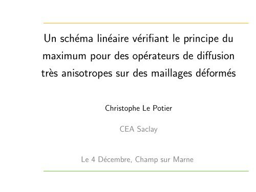
<strong>Un</strong> <strong>schéma</strong> <strong>linéaire</strong> <strong>vérifiant</strong> <strong>le</strong> <strong>principe</strong> <strong>du</strong><br />
<strong>maximum</strong> <strong>pour</strong> <strong>des</strong> opérateurs de diffusion<br />
très anisotropes sur <strong>des</strong> maillages déformés<br />
Christophe Le Potier<br />
CEA Saclay<br />
Le 4 Décembre, Champ sur Marne
Presentation<br />
Bibliographie<br />
Cas isotrope<br />
Cas anisotrope<br />
Propriétés <strong>du</strong> <strong>schéma</strong><br />
Résultats numériques<br />
Conclusion<br />
<strong>Un</strong> <strong>schéma</strong> <strong>linéaire</strong> <strong>vérifiant</strong> <strong>le</strong> <strong>principe</strong> <strong>du</strong> <strong>maximum</strong> <strong>pour</strong> <strong>des</strong> opérateurs de diffusion très anisotropes sur <strong>des</strong> maillages déformés, C. Le Potier p. 2
Présentation<br />
Considérons un domaine polygonal convexe Ω de frontière Γ de dimension 2. Nous<br />
simplifions <strong>le</strong> modè<strong>le</strong> de transport en supprimant la convection et la décroissance<br />
radioactive. Il s’écrit :<br />
( q = −D ∇C<br />
divq = S sur Ω<br />
avec C, la concentration de radionucléide, S, un terme source, D, une matrice<br />
(2,2) symétrique définie positive. D’autre part, <strong>des</strong> conditions aux limites <strong>du</strong> type<br />
Dirich<strong>le</strong>t sont imposées sur la frontière <strong>du</strong> domaine étudié.<br />
<strong>Un</strong> <strong>schéma</strong> <strong>linéaire</strong> <strong>vérifiant</strong> <strong>le</strong> <strong>principe</strong> <strong>du</strong> <strong>maximum</strong> <strong>pour</strong> <strong>des</strong> opérateurs de diffusion très anisotropes sur <strong>des</strong> maillages déformés, C. Le Potier p. 3<br />
(1)
Bibliographie (Schémas <strong>linéaire</strong>s )<br />
Cas isotrope: hypothèse géométrique. Par exemp<strong>le</strong>, <strong>pour</strong> <strong>des</strong> triang<strong>le</strong>s :<br />
θ1<br />
Condition d’ang<strong>le</strong> : θ1 + θ2 ≤ π <strong>pour</strong> E.F et <strong>le</strong>s V.F (VF4).<br />
Condition de Delaunay<br />
J. Xu, L. Zikatanov, A monotone finite e<strong>le</strong>ment scheme for convectiondiffusion<br />
equations, Math. Comp. 66 (228) (1999) 1429-1446<br />
<strong>Un</strong> <strong>schéma</strong> <strong>linéaire</strong> <strong>vérifiant</strong> <strong>le</strong> <strong>principe</strong> <strong>du</strong> <strong>maximum</strong> <strong>pour</strong> <strong>des</strong> opérateurs de diffusion très anisotropes sur <strong>des</strong> maillages déformés, C. Le Potier p. 4<br />
θ2
Bibliographie (Schémas non <strong>linéaire</strong>s)<br />
E. Burman et A. Ern (04) correction non <strong>linéaire</strong> <strong>des</strong> éléments finis.<br />
C.L.P (05) (VFMON) positif.<br />
K. Lipnikov, M. Shaskhov, D. Svyatskiy, Y. Vassi<strong>le</strong>vski(07)<br />
I. Kapyrin (07)<br />
G. Yuan, Z. Sheng, JCP (June 08)<br />
C.L.P(08), PMMD (FVCA5)<br />
<strong>Un</strong> <strong>schéma</strong> <strong>linéaire</strong> <strong>vérifiant</strong> <strong>le</strong> <strong>principe</strong> <strong>du</strong> <strong>maximum</strong> <strong>pour</strong> <strong>des</strong> opérateurs de diffusion très anisotropes sur <strong>des</strong> maillages déformés, C. Le Potier p. 5
En 1d<br />
Finite Volume Methods: R. Eymard, T. Gallouët, R. Herbin (2000)<br />
Maillage à pas non constant de [0,1] :<br />
... < xN = 1<br />
x0 = 0 < x1 < x 3 2<br />
h i+ 1 2<br />
... < xi < x i+ 1 2<br />
= xi+1 − xi, hi = x i+ 1 2<br />
ci = c(xi), Si = S(xi)<br />
Schéma volumes finis : F i+ 1 2<br />
F i+ 1 2<br />
= − ci+1 − ci<br />
h i+ 1 2<br />
− x i− 1 2<br />
− F i+ 1 2<br />
= hiSi<br />
<strong>Un</strong> <strong>schéma</strong> <strong>linéaire</strong> <strong>vérifiant</strong> <strong>le</strong> <strong>principe</strong> <strong>du</strong> <strong>maximum</strong> <strong>pour</strong> <strong>des</strong> opérateurs de diffusion très anisotropes sur <strong>des</strong> maillages déformés, C. Le Potier p. 6
En 1d<br />
Schéma VF : 1<br />
hi<br />
(− ci+1 − ci<br />
h i+ 1 2<br />
+ ci − ci−1<br />
h i− 1 2<br />
) = Si<br />
La solution ci converge vers la solution exacte cexa mais<br />
1<br />
hi<br />
(− ci+1 − ci<br />
h i+ 1 2<br />
Variante consistante:<br />
+ ci − ci−1<br />
h i− 1 2<br />
) n’approche pas en général ∂2 ci<br />
∂x 2<br />
4<br />
2hi + hi−1 + hi+1<br />
(− ci+1 − ci<br />
h i+ 1 2<br />
+ ci − ci−1<br />
h i− 1 2<br />
) = Si<br />
<strong>Un</strong> <strong>schéma</strong> <strong>linéaire</strong> <strong>vérifiant</strong> <strong>le</strong> <strong>principe</strong> <strong>du</strong> <strong>maximum</strong> <strong>pour</strong> <strong>des</strong> opérateurs de diffusion très anisotropes sur <strong>des</strong> maillages déformés, C. Le Potier p. 7
Cas isotrope<br />
Considérons un maillage de polygones quelconques de Ω constitué de Nma mail<strong>le</strong>s.<br />
Notons B = {Xi 1≤i≤Nma+N f } l’ensemb<strong>le</strong> constitué <strong>des</strong> Nma barycentres de<br />
chaque polygone et de Nf points situés sur la frontière ; (xi, yi) <strong>le</strong>s coordonnées<br />
de Xi.<br />
Soit une fonction c(x, y) de classe C 2 sur Ω. Le développement en série de Taylor<br />
autour <strong>du</strong> point (xi, yi) s’écrit :<br />
cj = ci + ∆xj<br />
∂ci<br />
∂x<br />
+ ∆yj<br />
∆xj∆yj<br />
∂ci<br />
∂y + ∆x2 j<br />
2<br />
∂ 2 ci<br />
∂x∂y<br />
∂ 2 ci<br />
∂x2 + ∆y2 j<br />
2<br />
q<br />
+ O(<br />
avec ∆xj = xj − xi, ∆yj = yj − yi, cj = c(xj, yj)<br />
∂ 2 ci<br />
+<br />
∂y2 ∆x 2 j + ∆y2 j<br />
<strong>Un</strong> <strong>schéma</strong> <strong>linéaire</strong> <strong>vérifiant</strong> <strong>le</strong> <strong>principe</strong> <strong>du</strong> <strong>maximum</strong> <strong>pour</strong> <strong>des</strong> opérateurs de diffusion très anisotropes sur <strong>des</strong> maillages déformés, C. Le Potier p. 8<br />
3<br />
)<br />
(2)
Cas isotrope<br />
Nous cherchons à approcher l’expression ∂2ci ∂x2 + ∂2ci P<br />
par<br />
∂y2 j=1,J zj(cj − ci),<br />
zj,j=1,J à déterminer. Système <strong>linéaire</strong> à résoudre : AZ = B, avec Z =<br />
(zj ) , J étant <strong>le</strong> nombre de points apparaissant dans <strong>le</strong> stencil <strong>du</strong> <strong>schéma</strong><br />
{1≤j≤J}<br />
A =<br />
0<br />
B<br />
@<br />
∆x1 .. ∆xJ<br />
∆y1 .. ∆yJ<br />
∆x 2 1<br />
2<br />
∆y 2 1<br />
..<br />
∆x 2 J<br />
2<br />
..<br />
∆x1∆y1 .. ∆xJ∆yJ<br />
<strong>Un</strong> <strong>schéma</strong> <strong>linéaire</strong> <strong>vérifiant</strong> <strong>le</strong> <strong>principe</strong> <strong>du</strong> <strong>maximum</strong> <strong>pour</strong> <strong>des</strong> opérateurs de diffusion très anisotropes sur <strong>des</strong> maillages déformés, C. Le Potier p. 9<br />
2<br />
∆y 2 J<br />
2<br />
1<br />
0<br />
C B<br />
C B<br />
C B<br />
C B<br />
C , B = B<br />
C B<br />
C B<br />
C B<br />
A @<br />
Différences finies généralisées : L. Gavete, M.L. Gavete, J.J. Benito (2003)<br />
0<br />
0<br />
1<br />
1<br />
0<br />
1<br />
C<br />
A<br />
(3)
Cas isotrope<br />
Par la suite, nous allons chercher une condition géométrique suffisante <strong>pour</strong> qu’il<br />
existe une solution positive non nul<strong>le</strong> au système précédent. Nous nous intéressons<br />
au système <strong>linéaire</strong> MU = B, avec U = (uj {1≤j≤J} ).<br />
M =<br />
0<br />
B<br />
@<br />
∆x1 .. ∆xJ<br />
∆y1 .. ∆yJ<br />
∆x 2 1 − ∆y 2 1 .. ∆x 2 J − ∆y 2 J<br />
∆x1∆y1 .. ∆xJ∆yJ<br />
<strong>Un</strong> <strong>schéma</strong> <strong>linéaire</strong> <strong>vérifiant</strong> <strong>le</strong> <strong>principe</strong> <strong>du</strong> <strong>maximum</strong> <strong>pour</strong> <strong>des</strong> opérateurs de diffusion très anisotropes sur <strong>des</strong> maillages déformés, C. Le Potier p. 10<br />
1<br />
0<br />
C B<br />
C B<br />
C B<br />
C , B = B<br />
C B<br />
A @<br />
0<br />
0<br />
0<br />
0<br />
1<br />
C<br />
A<br />
(4)
Cas isotrope<br />
∗X7<br />
∗X8<br />
∗X10<br />
∗X6<br />
∗X9<br />
∗X11<br />
∗X5<br />
y<br />
θ =<br />
∗X4<br />
∗X3<br />
3π<br />
8 π<br />
θ =<br />
4<br />
Xi<br />
∗X12 ∗X13 ∗X14<br />
<strong>Un</strong> <strong>schéma</strong> <strong>linéaire</strong> <strong>vérifiant</strong> <strong>le</strong> <strong>principe</strong> <strong>du</strong> <strong>maximum</strong> <strong>pour</strong> <strong>des</strong> opérateurs de diffusion très anisotropes sur <strong>des</strong> maillages déformés, C. Le Potier p. 11<br />
∗X1<br />
∗X2<br />
∗X16<br />
θ = π<br />
8<br />
x<br />
∗X15 θ = − π<br />
8<br />
θ = − π<br />
4<br />
θ = − 3π<br />
8<br />
16 secteurs autour <strong>du</strong> point Xi
Cas isotrope<br />
Proposition S’il existe un ensemb<strong>le</strong> de points Xj ∈ B satisfaisant la propriété<br />
décrite sur la figure précédente, alors il existe une solution U non nul<strong>le</strong> qui<br />
est positive.<br />
Preuve<br />
Le point Xi étant à l’intérieur <strong>du</strong> quadrang<strong>le</strong> (X1, X2, X9, X10), il existe 4 coefficients<br />
positifs (s1,1, s2,1, s9,1, s10,1) tels que :<br />
s1,1 XiX1 + s2,1 XiX2 + s9,1 XiX9 + s10,1 XiX10 = 0.<br />
<strong>Un</strong> <strong>schéma</strong> <strong>linéaire</strong> <strong>vérifiant</strong> <strong>le</strong> <strong>principe</strong> <strong>du</strong> <strong>maximum</strong> <strong>pour</strong> <strong>des</strong> opérateurs de diffusion très anisotropes sur <strong>des</strong> maillages déformés, C. Le Potier p. 12
Cas isotrope<br />
8<br />
><<br />
>:<br />
s1,1∆x1 + s2,1∆x2 + s9,1∆x9 + s10,1∆x10 = 0<br />
s1,1∆y1 + s2,1∆y2 + s9,1∆y9 + s10,1∆y10 = 0<br />
s1,1(∆x 2 1 − ∆y 2 1) + s2,1(∆x 2 2 − ∆y 2 2)+<br />
s9,1(∆x 2 9 − ∆y 2 9) + s10,1(∆x 2 10 − ∆y 2 10) ≥ 0<br />
s1,1∆x1∆y1 + s2,1∆x2∆y2 + s9,1∆x9∆y9 + s10,1∆x10∆y10 ≥ 0<br />
car dans <strong>le</strong> voisinage de la droite θ = π<br />
8 , ∆x2 j − ∆y 2 j ≥ 0 et ∆xj∆yj ≥ 0.<br />
On définit alors 3 autres combinaisons <strong>linéaire</strong>s sj,k {j=1,16,k=1,4} qui vérifient <strong>le</strong>s<br />
2 premières équations (autour <strong>des</strong> droites θ = − π 3π<br />
, θ =<br />
8 8<br />
Notons Exp3k = P<br />
j=1,16 sj,k(∆x 2 j −∆y 2 j) et Exp4k = P<br />
k = 1, 4.<br />
et θ = −3π<br />
8 ).<br />
<strong>Un</strong> <strong>schéma</strong> <strong>linéaire</strong> <strong>vérifiant</strong> <strong>le</strong> <strong>principe</strong> <strong>du</strong> <strong>maximum</strong> <strong>pour</strong> <strong>des</strong> opérateurs de diffusion très anisotropes sur <strong>des</strong> maillages déformés, C. Le Potier p. 13<br />
(5)<br />
j=1,16 sj,k∆xj∆yj où
Cas isotrope<br />
Exp3k Exp4k<br />
k = 1 ≥ 0 ≥ 0<br />
Exp3k Exp4k<br />
k = 3 ≤ 0 ≥ 0<br />
Exp3k Exp4k<br />
k = 2 ≥ 0 ≤ 0<br />
Exp3k Exp4k<br />
k = 4 ≤ 0 ≤ 0<br />
Il existe deux réels positifs α1 et α3 tels que α1Exp31 + α3Exp33 = 0 et<br />
α1Exp41 + α3Exp43 ≥ 0.<br />
De même, il existe α2 et α4, réels positifs tels que α2Exp32 + α4Exp34 = 0 et<br />
α2Exp42 + α4Exp44 ≤ 0.<br />
<strong>le</strong>s 3 premières équations sont vérifiées.<br />
<strong>Un</strong> <strong>schéma</strong> <strong>linéaire</strong> <strong>vérifiant</strong> <strong>le</strong> <strong>principe</strong> <strong>du</strong> <strong>maximum</strong> <strong>pour</strong> <strong>des</strong> opérateurs de diffusion très anisotropes sur <strong>des</strong> maillages déformés, C. Le Potier p. 14
Cas isotrope<br />
Il existe donc β1 et β2 réels positifs tels que<br />
( β1(α1Exp31 + α3Exp33) + β2(α2Exp32 + α4Exp34) = 0<br />
β1(α1Exp41 + α3Exp43) + β2(α2Exp42 + α4Exp44) = 0<br />
Les 4 équations sont vérifiées.<br />
Il existe donc 16 va<strong>le</strong>urs uj,{j=1,16} positives non toutes nul<strong>le</strong>s <strong>vérifiant</strong> <strong>le</strong> système<br />
<strong>linéaire</strong> MU = B. On pose alors Z = (zj {j=1,16} ) qui vérifie Z = νU avec<br />
2<br />
ν = P<br />
j=1,16 uj∆x2 = P<br />
j<br />
par P<br />
j=1,16 zj(cj − ci).<br />
2<br />
j=1,16 uj∆y 2 j<br />
<strong>Un</strong> <strong>schéma</strong> <strong>linéaire</strong> <strong>vérifiant</strong> <strong>le</strong> <strong>principe</strong> <strong>du</strong> <strong>maximum</strong> <strong>pour</strong> <strong>des</strong> opérateurs de diffusion très anisotropes sur <strong>des</strong> maillages déformés, C. Le Potier p. 15<br />
(6)<br />
et on approche l’expression ∂2ci ∂x2 + ∂2ci ∂y2
Cas anisotrope<br />
Le tenseur D symétrique est diagonalisab<strong>le</strong>.<br />
(λ1, λ2) <strong>le</strong>s 2 va<strong>le</strong>urs propres<br />
r<br />
λ2<br />
= arctan( )<br />
θλ1,λ2<br />
λ1<br />
(Xi, X, Y ) X et Y , vecteurs propres normés<br />
16 secteurs, θ = θλ1,λ2<br />
2<br />
θ = − π<br />
4<br />
− θλ1,λ2<br />
2<br />
, θ = − θλ1,λ2<br />
2<br />
, θ = π<br />
4<br />
+ θλ1,λ2<br />
2<br />
, θ = θλ1,λ2, θ = −θλ1,λ2, θ = 0, θ = π<br />
2 .<br />
On suppose qu’il existe Xj ∈ B dans chaque secteur. La proposition précédente<br />
se généralise.<br />
<strong>Un</strong> <strong>schéma</strong> <strong>linéaire</strong> <strong>vérifiant</strong> <strong>le</strong> <strong>principe</strong> <strong>du</strong> <strong>maximum</strong> <strong>pour</strong> <strong>des</strong> opérateurs de diffusion très anisotropes sur <strong>des</strong> maillages déformés, C. Le Potier p. 16<br />
,
Cas anisotrope<br />
∗X7<br />
∗X8<br />
∗X10<br />
∗X6<br />
∗X9<br />
∗X11<br />
∗X5<br />
Y<br />
∗X4<br />
Xi<br />
∗X3<br />
∗X2<br />
θ = θλ1,λ2<br />
θ =<br />
θ = θλ1,λ2<br />
2<br />
π θλ1,λ2<br />
+<br />
4 2<br />
<strong>Un</strong> <strong>schéma</strong> <strong>linéaire</strong> <strong>vérifiant</strong> <strong>le</strong> <strong>principe</strong> <strong>du</strong> <strong>maximum</strong> <strong>pour</strong> <strong>des</strong> opérateurs de diffusion très anisotropes sur <strong>des</strong> maillages déformés, C. Le Potier p. 17<br />
∗X1<br />
∗X15<br />
∗X16<br />
X<br />
θ = − θλ1,λ2<br />
2<br />
θ = −θλ1,λ2<br />
∗X12 ∗X13 ∗X14<br />
θ = − π θλ1,λ2<br />
−<br />
4 2<br />
16 secteurs autour <strong>du</strong> point Xi
D =<br />
Cas hétérogène<br />
D1,1(x, y) D2,1(x, y)<br />
D2,1(x, y) D2,2(x, y)<br />
D1,1(x, y), D2,2(x, y) et D2,1(x, y) suffisamment régulières.<br />
8<br />
><<br />
>:<br />
!<br />
.<br />
D1,1(x, y) ∂2C ∂x2 + 2D2,1(x, y) ∂2C ∂x∂y + D2,2(x, y) ∂2C +<br />
∂y2 ∂D1,1(x, y) ∂C(x, y)<br />
+<br />
∂x ∂x<br />
∂D2,1(x, y) ∂C(x,y)<br />
∂x ∂y +<br />
∂D2,1(x, y) ∂C(x, y)<br />
+<br />
∂y ∂x<br />
∂D2,2(x, y) ∂C(x,y)<br />
= −S<br />
∂y ∂y<br />
Problème convectif-diffusif.<br />
Terme diffusif : <strong>le</strong>s vecteurs propres dépendent de x,y. idem cas homogène<br />
anisotrope.<br />
<strong>Un</strong> <strong>schéma</strong> <strong>linéaire</strong> <strong>vérifiant</strong> <strong>le</strong> <strong>principe</strong> <strong>du</strong> <strong>maximum</strong> <strong>pour</strong> <strong>des</strong> opérateurs de diffusion très anisotropes sur <strong>des</strong> maillages déformés, C. Le Potier p. 18<br />
(7)
Cas hétérogène<br />
Terme convectif<br />
∂C(x, y)<br />
(<strong>pour</strong> ): MxUx = Bx, avec Ux = (u<br />
∂x<br />
x j ), J étant <strong>le</strong> nombre de<br />
{1≤j≤J}<br />
points apparaissant dans <strong>le</strong> stencil <strong>du</strong> <strong>schéma</strong>.<br />
Mx =<br />
∆x1 .. ∆xJ<br />
∆y1 .. ∆yJ<br />
∗X2<br />
∗X3<br />
y<br />
Xi<br />
<strong>Un</strong> <strong>schéma</strong> <strong>linéaire</strong> <strong>vérifiant</strong> <strong>le</strong> <strong>principe</strong> <strong>du</strong> <strong>maximum</strong> <strong>pour</strong> <strong>des</strong> opérateurs de diffusion très anisotropes sur <strong>des</strong> maillages déformés, C. Le Potier p. 19<br />
!<br />
∗X1<br />
∗X4<br />
, Bx =<br />
4 secteurs autour <strong>du</strong> point Xi<br />
x<br />
valx<br />
0<br />
!<br />
(8)
Cas hétérogène<br />
Proposition : s’il existe un ensemb<strong>le</strong> de points Xj ∈ B satisfaisant la propriété<br />
décrite sur la figure précédente, alors il existe Ux, non nul positif tels que<br />
MxUx = Bx<br />
∂C(x, y)<br />
∂x<br />
approché par P<br />
même propriété <strong>pour</strong><br />
∂C(x, y)<br />
∂y<br />
j=1,4 uj,x(cj − ci)<br />
Schéma d’ordre 1 type <strong>schéma</strong> décentré.<br />
Cas diffusif dominant : ordre 2 <strong>pour</strong> <strong>le</strong> terme convectif.<br />
<strong>Un</strong> <strong>schéma</strong> <strong>linéaire</strong> <strong>vérifiant</strong> <strong>le</strong> <strong>principe</strong> <strong>du</strong> <strong>maximum</strong> <strong>pour</strong> <strong>des</strong> opérateurs de diffusion très anisotropes sur <strong>des</strong> maillages déformés, C. Le Potier p. 20
Propriétés : consistance<br />
Soit Ch <strong>le</strong>s va<strong>le</strong>urs de C en Xi, Sh <strong>le</strong>s va<strong>le</strong>urs de S en Xi et Ah la matrice associée<br />
au <strong>schéma</strong> tel que AhCh = Sh.<br />
Pour chaque point à l’intérieur <strong>du</strong> maillage, ajout d’un nombre suffisant de<br />
points sur la frontière tel que la propriété décrite sur la figure précédente<br />
soit vérifiée.<br />
rmaxi rayon minimum <strong>du</strong> cerc<strong>le</strong> tel que <strong>le</strong>s 16 points Xj ∈ B soient à<br />
l’intérieur de ce cerc<strong>le</strong>.<br />
Hypothèse : rmaxi tend vers 0 lorsque l’on raffine <strong>le</strong> maillage.<br />
Comme X<br />
zj ≤ 2<br />
∆x 2 j<br />
j=1,16<br />
zj<br />
∆x 2 j<br />
2<br />
et zj ≤ 2<br />
∆y 2 j<br />
= X<br />
.<br />
j=1,16<br />
zj<br />
∆y 2 j<br />
2 = 1 avec zj ≥ 0, alors<br />
Donc P<br />
j=1,16 zj(cj − ci) = ∂2ci ∂x2 + ∂2ci X<br />
+<br />
∂y2 j=1,16<br />
q<br />
zjO( ∆x2 j + ∆y2 3<br />
j ) =<br />
∂ 2 ci<br />
∂x 2 + ∂2 ci<br />
∂y 2 + O(rmaxi) ce qui prouve la consistance <strong>du</strong> <strong>schéma</strong>.<br />
<strong>Un</strong> <strong>schéma</strong> <strong>linéaire</strong> <strong>vérifiant</strong> <strong>le</strong> <strong>principe</strong> <strong>du</strong> <strong>maximum</strong> <strong>pour</strong> <strong>des</strong> opérateurs de diffusion très anisotropes sur <strong>des</strong> maillages déformés, C. Le Potier p. 21
Propriétés <strong>du</strong> <strong>schéma</strong> : consistance<br />
Remarque<br />
On choisit <strong>le</strong>s Xj ∈ B <strong>le</strong>s plus proches de Xi appartenant aux 16 secteurs<br />
de la figure précédente.<br />
Pour un maillage de parallélogrammes d’ang<strong>le</strong> aigu ν dont <strong>le</strong>s côtés sont<br />
de longueur r, il existe une fonction positive g et un cerc<strong>le</strong> de rayon g(ν)r<br />
tels que <strong>le</strong>s points de la figure précédente soient à l’intérieur de ce cerc<strong>le</strong>.<br />
La fonction g tend vers +∞ lorsque ν tend vers 0. Le <strong>schéma</strong> reste<br />
consistant mais perd en précision.<br />
rmaxi tend vers zéro lorsqu’on raffine <strong>le</strong> maillage.<br />
Même propriété, lorsque la régularité ne varie pas dans une convergence en<br />
maillage<br />
<strong>Un</strong> <strong>schéma</strong> <strong>linéaire</strong> <strong>vérifiant</strong> <strong>le</strong> <strong>principe</strong> <strong>du</strong> <strong>maximum</strong> <strong>pour</strong> <strong>des</strong> opérateurs de diffusion très anisotropes sur <strong>des</strong> maillages déformés, C. Le Potier p. 22
Propriétés : <strong>principe</strong> <strong>du</strong> <strong>maximum</strong><br />
Si la proposition précédente est vérifiée, <strong>le</strong>s coefficients zj sont tous<br />
positifs.<br />
La matrice Ah est irré<strong>du</strong>ctib<strong>le</strong>.<br />
La matrice Ah est une M-matrice.<br />
Principe <strong>du</strong> <strong>maximum</strong>.<br />
<strong>Un</strong> <strong>schéma</strong> <strong>linéaire</strong> <strong>vérifiant</strong> <strong>le</strong> <strong>principe</strong> <strong>du</strong> <strong>maximum</strong> <strong>pour</strong> <strong>des</strong> opérateurs de diffusion très anisotropes sur <strong>des</strong> maillages déformés, C. Le Potier p. 23
Propriétés : stabilité et convergence<br />
Pour v = −(x 2 + y 2 ), Ahv = A0 = 2D1,1 + 2D2,2, D1,1 et D2,2 sont <strong>le</strong>s<br />
termes de la diagona<strong>le</strong> de D.<br />
Avec <strong>principe</strong> <strong>du</strong> <strong>maximum</strong>, (Thèse I. Fail<strong>le</strong> : (I.F.P.)) ||A −1<br />
h ||∞ ≤ G où<br />
G = ||v||∞<br />
A0<br />
est un coefficient strictement positif indépendant de<br />
rmax = max{i=1,Nma}rmaxi.<br />
Si <strong>le</strong>s hypothèses de la figure précédente sont satisfaites et si <strong>pour</strong> chaque<br />
point Xi ∈ B à l’intérieur <strong>du</strong> maillage, rmaxi tend vers zéro lorsqu’on<br />
raffine <strong>le</strong> maillage, <strong>le</strong> <strong>schéma</strong> (DFPMD) est convergent en norme infini car<br />
il est consistant et stab<strong>le</strong>. Il est au moins d’ordre 1.<br />
<strong>Un</strong> <strong>schéma</strong> <strong>linéaire</strong> <strong>vérifiant</strong> <strong>le</strong> <strong>principe</strong> <strong>du</strong> <strong>maximum</strong> <strong>pour</strong> <strong>des</strong> opérateurs de diffusion très anisotropes sur <strong>des</strong> maillages déformés, C. Le Potier p. 24
Remarque<br />
”On the non existence of monotone linear schema for some linear parabolic equations<br />
Comptes Ren<strong>du</strong>s Mathematique, Volume 340, Issue 5, 1 March 2005, Pages<br />
399-404 Christophe Buet, Stéphane Cordier”<br />
VF9 ou DF9 avec tenseurs anisotropes.<br />
DFPMD est une solution.<br />
Solution non <strong>linéaire</strong>.<br />
<strong>Un</strong> <strong>schéma</strong> <strong>linéaire</strong> <strong>vérifiant</strong> <strong>le</strong> <strong>principe</strong> <strong>du</strong> <strong>maximum</strong> <strong>pour</strong> <strong>des</strong> opérateurs de diffusion très anisotropes sur <strong>des</strong> maillages déformés, C. Le Potier p. 25
Remarque<br />
Schéma en général non conservatif (sauf cas particulier) qui converge quand<br />
même!<br />
<strong>Un</strong> <strong>schéma</strong> <strong>linéaire</strong> <strong>vérifiant</strong> <strong>le</strong> <strong>principe</strong> <strong>du</strong> <strong>maximum</strong> <strong>pour</strong> <strong>des</strong> opérateurs de diffusion très anisotropes sur <strong>des</strong> maillages déformés, C. Le Potier p. 26
Résultats numériques<br />
Solution analytique stationnaire<br />
Exemp<strong>le</strong> de E. Burman et A. Ern<br />
Ω =]0,1.0[×]0,0.3[<br />
Tenseur isotrope<br />
Rectang<strong>le</strong>s découpés en 4 triang<strong>le</strong>s<br />
Condition de Delaunay non vérifiée<br />
Conditions aux limites de Dirich<strong>le</strong>t : C = 0<br />
Can(x, y) = sin(πx)sin((π/0.3)y)<br />
S = −divD ∇Can<br />
<strong>Un</strong> <strong>schéma</strong> <strong>linéaire</strong> <strong>vérifiant</strong> <strong>le</strong> <strong>principe</strong> <strong>du</strong> <strong>maximum</strong> <strong>pour</strong> <strong>des</strong> opérateurs de diffusion très anisotropes sur <strong>des</strong> maillages déformés, C. Le Potier p. 27
Résultats numériques<br />
Maillage de 64 triang<strong>le</strong>s.<br />
<strong>Un</strong> <strong>schéma</strong> <strong>linéaire</strong> <strong>vérifiant</strong> <strong>le</strong> <strong>principe</strong> <strong>du</strong> <strong>maximum</strong> <strong>pour</strong> <strong>des</strong> opérateurs de diffusion très anisotropes sur <strong>des</strong> maillages déformés, C. Le Potier p. 28
Résultats numériques<br />
h,k<br />
1 0.3<br />
, 4 4<br />
1 0.3<br />
, 8 8<br />
1 0.3<br />
, 16 16<br />
1 0.3<br />
, 32 32<br />
Nma 64 256 1024 4096<br />
Erreur L 2<br />
9,0.10 −2<br />
2, 8.10 −2<br />
8, 9.10 −3<br />
4,4.10 −3<br />
Ordre 1.66 1.68 1.0<br />
h,k<br />
1 0.3<br />
, 64 64<br />
1 0.3<br />
, 128 128<br />
1 0.3<br />
, 256 256<br />
Nma 16384 65536 262144<br />
Erreur L 2<br />
1,8.10 −3<br />
8, 1.10 −4<br />
4, 0.10 −4<br />
Ordre 1.32 1.12 1.04<br />
Erreur L 2 et ordre en fonction <strong>du</strong> pas de discrétisation<br />
<strong>Un</strong> <strong>schéma</strong> <strong>linéaire</strong> <strong>vérifiant</strong> <strong>le</strong> <strong>principe</strong> <strong>du</strong> <strong>maximum</strong> <strong>pour</strong> <strong>des</strong> opérateurs de diffusion très anisotropes sur <strong>des</strong> maillages déformés, C. Le Potier p. 29
Résultats numériques<br />
Solution stationnaire avec terme source discontinue<br />
Exemp<strong>le</strong> de E. Burman et A. Ern<br />
Ω =]0,1.0[×]0,0.3[<br />
Cas isotrope<br />
Rectang<strong>le</strong>s découpés en 4 triang<strong>le</strong>s<br />
Conditions aux limites de Dirich<strong>le</strong>t : C = 0.<br />
S = 1 sur ]0., 0.5[×]0.,0.075[ et 0 sinon.<br />
EFMH/VF(MPFA)/DFPMD (F. Dabbène, G. Bernard-Michel, S. Gounand,<br />
C.L.P.)<br />
<strong>Un</strong> <strong>schéma</strong> <strong>linéaire</strong> <strong>vérifiant</strong> <strong>le</strong> <strong>principe</strong> <strong>du</strong> <strong>maximum</strong> <strong>pour</strong> <strong>des</strong> opérateurs de diffusion très anisotropes sur <strong>des</strong> maillages déformés, C. Le Potier p. 30
Résultats numériques<br />
Maillage de 64 mail<strong>le</strong>s et source.<br />
SCAL<br />
> 0.00E+00<br />
< 1.00E+00<br />
7.81E−03<br />
5.47E−02<br />
0.10<br />
0.15<br />
0.20<br />
0.24<br />
0.29<br />
0.34<br />
0.38<br />
0.43<br />
0.48<br />
0.52<br />
0.57<br />
0.62<br />
0.66<br />
0.71<br />
0.76<br />
0.80<br />
0.85<br />
0.90<br />
0.95<br />
0.99<br />
<strong>Un</strong> <strong>schéma</strong> <strong>linéaire</strong> <strong>vérifiant</strong> <strong>le</strong> <strong>principe</strong> <strong>du</strong> <strong>maximum</strong> <strong>pour</strong> <strong>des</strong> opérateurs de diffusion très anisotropes sur <strong>des</strong> maillages déformés, C. Le Potier p. 31
Résultats numériques<br />
SCAL<br />
>−1.94E−04<br />
< 2.83E−03<br />
−1.71E−04<br />
−2.89E−05<br />
1.13E−04<br />
2.55E−04<br />
3.97E−04<br />
5.39E−04<br />
6.81E−04<br />
8.22E−04<br />
9.64E−04<br />
1.11E−03<br />
1.25E−03<br />
1.39E−03<br />
1.53E−03<br />
1.67E−03<br />
1.82E−03<br />
1.96E−03<br />
2.10E−03<br />
2.24E−03<br />
2.38E−03<br />
2.53E−03<br />
2.67E−03<br />
2.81E−03<br />
EFMH (concentration et lieu <strong>des</strong> va<strong>le</strong>urs négatives) 64 mail<strong>le</strong>s, va<strong>le</strong>ur minimum<br />
−1.94 × 10 −4 , 12 % d’oscillations<br />
<strong>Un</strong> <strong>schéma</strong> <strong>linéaire</strong> <strong>vérifiant</strong> <strong>le</strong> <strong>principe</strong> <strong>du</strong> <strong>maximum</strong> <strong>pour</strong> <strong>des</strong> opérateurs de diffusion très anisotropes sur <strong>des</strong> maillages déformés, C. Le Potier p. 32<br />
SCAL<br />
> 0.00E+00<br />
< 1.00E+00<br />
7.81E−03<br />
5.47E−02<br />
0.10<br />
0.15<br />
0.20<br />
0.24<br />
0.29<br />
0.34<br />
0.38<br />
0.43<br />
0.48<br />
0.52<br />
0.57<br />
0.62<br />
0.66<br />
0.71<br />
0.76<br />
0.80<br />
0.85<br />
0.90<br />
0.95<br />
0.99
Résultats numériques<br />
SCAL<br />
>−3.96E−03<br />
< 8.44E−02<br />
−3.27E−03<br />
8.72E−04<br />
5.02E−03<br />
9.16E−03<br />
1.33E−02<br />
1.74E−02<br />
2.16E−02<br />
2.57E−02<br />
2.99E−02<br />
3.40E−02<br />
3.82E−02<br />
4.23E−02<br />
4.64E−02<br />
5.06E−02<br />
5.47E−02<br />
5.89E−02<br />
6.30E−02<br />
6.72E−02<br />
7.13E−02<br />
7.55E−02<br />
7.96E−02<br />
8.37E−02<br />
VF(MPFA) (concentration et lieu <strong>des</strong> va<strong>le</strong>urs négatives) 64 mail<strong>le</strong>s, va<strong>le</strong>ur minimum<br />
−3.96 × 10 −2 , 17 % d’oscillations<br />
<strong>Un</strong> <strong>schéma</strong> <strong>linéaire</strong> <strong>vérifiant</strong> <strong>le</strong> <strong>principe</strong> <strong>du</strong> <strong>maximum</strong> <strong>pour</strong> <strong>des</strong> opérateurs de diffusion très anisotropes sur <strong>des</strong> maillages déformés, C. Le Potier p. 33<br />
SCAL<br />
> 0.00E+00<br />
< 1.00E+00<br />
0.0<br />
5.00E−02<br />
0.10<br />
0.15<br />
0.20<br />
0.25<br />
0.30<br />
0.35<br />
0.40<br />
0.45<br />
0.50<br />
0.55<br />
0.60<br />
0.65<br />
0.70<br />
0.75<br />
0.80<br />
0.85<br />
0.90<br />
0.95<br />
1.0
Résultats numériques<br />
DFPMD (concentration) 64 mail<strong>le</strong>s<br />
SCAL<br />
> 4.41E−07<br />
< 3.12E−03<br />
2.48E−05<br />
1.71E−04<br />
3.18E−04<br />
4.64E−04<br />
6.10E−04<br />
7.57E−04<br />
9.03E−04<br />
1.05E−03<br />
1.20E−03<br />
1.34E−03<br />
1.49E−03<br />
1.63E−03<br />
1.78E−03<br />
1.93E−03<br />
2.07E−03<br />
2.22E−03<br />
2.37E−03<br />
2.51E−03<br />
2.66E−03<br />
2.81E−03<br />
2.95E−03<br />
3.10E−03<br />
<strong>Un</strong> <strong>schéma</strong> <strong>linéaire</strong> <strong>vérifiant</strong> <strong>le</strong> <strong>principe</strong> <strong>du</strong> <strong>maximum</strong> <strong>pour</strong> <strong>des</strong> opérateurs de diffusion très anisotropes sur <strong>des</strong> maillages déformés, C. Le Potier p. 34
Résultats numériques<br />
Solution analytique stationnaire<br />
Inspiré par <strong>le</strong> benchmark de FVCA5 (R. Herbin et F. Hubert)<br />
Ω =]0,1.0[×]0,1.0[<br />
D = Rθ<br />
1 0<br />
0 10 −3<br />
Conditions aux limites de Dirich<strong>le</strong>t : C = 0<br />
!<br />
Can(x, y) = sin(πx)sin(πy)<br />
S = −divD ∇Can<br />
Maillage de carrés.<br />
Rθ −1 , Rθ, rotation d’ang<strong>le</strong> θ = −67.5 degrés<br />
<strong>Un</strong> <strong>schéma</strong> <strong>linéaire</strong> <strong>vérifiant</strong> <strong>le</strong> <strong>principe</strong> <strong>du</strong> <strong>maximum</strong> <strong>pour</strong> <strong>des</strong> opérateurs de diffusion très anisotropes sur <strong>des</strong> maillages déformés, C. Le Potier p. 35
Résultats numériques<br />
h<br />
1<br />
4<br />
1<br />
8<br />
Nma 16 64 256 1024 4096<br />
Erreur L 2<br />
5,2.10 −1<br />
4, 7.10 −1<br />
<strong>Un</strong> <strong>schéma</strong> <strong>linéaire</strong> <strong>vérifiant</strong> <strong>le</strong> <strong>principe</strong> <strong>du</strong> <strong>maximum</strong> <strong>pour</strong> <strong>des</strong> opérateurs de diffusion très anisotropes sur <strong>des</strong> maillages déformés, C. Le Potier p. 36<br />
1<br />
16<br />
2, 6.10 −1<br />
1<br />
32<br />
7,1.1 −2<br />
1<br />
64<br />
2, 5.10 −2<br />
Ordre 0.14 0.85 1.87 1.51<br />
h<br />
1<br />
128<br />
1<br />
256<br />
1<br />
512<br />
Nma 16384 65536 262144<br />
Erreur L 2<br />
7,7.10 −3<br />
2, 1.10 −3<br />
5, 6.10 −4<br />
Ordre 1.68 1.85 1.92<br />
Erreur L 2 et ordre en fonction <strong>du</strong> pas de discrétisation
Résultats numériques<br />
Solution stationnaire avec terme source discontinue<br />
Ω =]0,1.0[×]0,1.0[<br />
D = Rθ<br />
1 0<br />
0 10 −3<br />
!<br />
Conditions aux limites de Dirich<strong>le</strong>t : C = 0.<br />
S = 1 sur ]0.25,0.75[×]0.25,0.75[ et 0 sinon.<br />
Maillage de carrés.<br />
Rθ −1 , Rθ est la rotation d’ang<strong>le</strong> θ = −67.5 degrés<br />
<strong>Un</strong> <strong>schéma</strong> <strong>linéaire</strong> <strong>vérifiant</strong> <strong>le</strong> <strong>principe</strong> <strong>du</strong> <strong>maximum</strong> <strong>pour</strong> <strong>des</strong> opérateurs de diffusion très anisotropes sur <strong>des</strong> maillages déformés, C. Le Potier p. 37
Résultats numériques<br />
SCAL<br />
>−7.63E−03<br />
< 1.13E−01<br />
−6.68E−03<br />
−1.01E−03<br />
4.67E−03<br />
1.03E−02<br />
1.60E−02<br />
2.17E−02<br />
2.74E−02<br />
3.30E−02<br />
3.87E−02<br />
4.44E−02<br />
5.01E−02<br />
5.57E−02<br />
6.14E−02<br />
6.71E−02<br />
7.28E−02<br />
7.84E−02<br />
8.41E−02<br />
8.98E−02<br />
9.54E−02<br />
0.10<br />
0.11<br />
0.11<br />
EFMH (concentration et lieu <strong>des</strong> va<strong>le</strong>urs négatives) 16384 mail<strong>le</strong>s, va<strong>le</strong>ur minimum<br />
−7.6 × 10 −3 , 19 % d’oscillations<br />
<strong>Un</strong> <strong>schéma</strong> <strong>linéaire</strong> <strong>vérifiant</strong> <strong>le</strong> <strong>principe</strong> <strong>du</strong> <strong>maximum</strong> <strong>pour</strong> <strong>des</strong> opérateurs de diffusion très anisotropes sur <strong>des</strong> maillages déformés, C. Le Potier p. 38<br />
SCAL<br />
> 0.00E+00<br />
< 1.00E+00<br />
7.81E−03<br />
5.47E−02<br />
0.10<br />
0.15<br />
0.20<br />
0.24<br />
0.29<br />
0.34<br />
0.38<br />
0.43<br />
0.48<br />
0.52<br />
0.57<br />
0.62<br />
0.66<br />
0.71<br />
0.76<br />
0.80<br />
0.85<br />
0.90<br />
0.95<br />
0.99
Résultats numériques<br />
SCAL<br />
>−3.08E−05<br />
< 1.10E−01<br />
8.27E−04<br />
5.98E−03<br />
1.11E−02<br />
1.63E−02<br />
2.14E−02<br />
2.66E−02<br />
3.17E−02<br />
3.69E−02<br />
4.20E−02<br />
4.72E−02<br />
5.23E−02<br />
5.75E−02<br />
6.26E−02<br />
6.78E−02<br />
7.29E−02<br />
7.81E−02<br />
8.32E−02<br />
8.84E−02<br />
9.35E−02<br />
9.87E−02<br />
0.10<br />
0.11<br />
VFSYM (concentration et lieu <strong>des</strong> va<strong>le</strong>urs négatives) 16384 mail<strong>le</strong>s, va<strong>le</strong>ur minimum<br />
−3.0 × 10 −5 , 7 % d’oscillations<br />
<strong>Un</strong> <strong>schéma</strong> <strong>linéaire</strong> <strong>vérifiant</strong> <strong>le</strong> <strong>principe</strong> <strong>du</strong> <strong>maximum</strong> <strong>pour</strong> <strong>des</strong> opérateurs de diffusion très anisotropes sur <strong>des</strong> maillages déformés, C. Le Potier p. 39<br />
SCAL<br />
> 0.00E+00<br />
< 1.00E+00<br />
7.81E−03<br />
5.47E−02<br />
0.10<br />
0.15<br />
0.20<br />
0.24<br />
0.29<br />
0.34<br />
0.38<br />
0.43<br />
0.48<br />
0.52<br />
0.57<br />
0.62<br />
0.66<br />
0.71<br />
0.76<br />
0.80<br />
0.85<br />
0.90<br />
0.95<br />
0.99
Résultats numériques<br />
DFPMD (concentration) 16384 mail<strong>le</strong>s<br />
SCAL<br />
> 0.00E+00<br />
< 1.10E−01<br />
8.60E−04<br />
6.02E−03<br />
1.12E−02<br />
1.63E−02<br />
2.15E−02<br />
2.66E−02<br />
3.18E−02<br />
3.70E−02<br />
4.21E−02<br />
4.73E−02<br />
5.24E−02<br />
5.76E−02<br />
6.27E−02<br />
6.79E−02<br />
7.31E−02<br />
7.82E−02<br />
8.34E−02<br />
8.85E−02<br />
9.37E−02<br />
9.89E−02<br />
0.10<br />
0.11<br />
<strong>Un</strong> <strong>schéma</strong> <strong>linéaire</strong> <strong>vérifiant</strong> <strong>le</strong> <strong>principe</strong> <strong>du</strong> <strong>maximum</strong> <strong>pour</strong> <strong>des</strong> opérateurs de diffusion très anisotropes sur <strong>des</strong> maillages déformés, C. Le Potier p. 40
Conclusion<br />
Convergence numérique vérifiée.<br />
Système <strong>linéaire</strong> faci<strong>le</strong> à inverser (Pas de Newton ou de point fixe).<br />
Prix de la méthode : ordre entre 1 et 2 en espace sur <strong>le</strong>s maillages<br />
déformés et <strong>le</strong>s tenseurs très anisotropes.<br />
Pour <strong>des</strong> maillages déformés avec tenseurs anisotropes, <strong>schéma</strong> ordre 1 :<br />
<strong>linéaire</strong>, <strong>schéma</strong> ordre 2 : non <strong>linéaire</strong><br />
Propriétés proches <strong>des</strong> <strong>schéma</strong>s approximant un terme convectif. Ordre 1 :<br />
<strong>schéma</strong> TVD, ordre 2 : <strong>schéma</strong> non <strong>linéaire</strong>.<br />
<strong>Un</strong> <strong>schéma</strong> <strong>linéaire</strong> <strong>vérifiant</strong> <strong>le</strong> <strong>principe</strong> <strong>du</strong> <strong>maximum</strong> <strong>pour</strong> <strong>des</strong> opérateurs de diffusion très anisotropes sur <strong>des</strong> maillages déformés, C. Le Potier p. 41