Evaluation de la performance et analyse du ... - IUT Bordeaux 1...
Evaluation de la performance et analyse du ... - IUT Bordeaux 1...
Evaluation de la performance et analyse du ... - IUT Bordeaux 1...

Create successful ePaper yourself
Turn your PDF publications into a flip-book with our unique Google optimized e-Paper software.
6 25 e rencontres <strong>de</strong> l’AUGC, 23-25 mai 2007, Bor<strong>de</strong>aux<br />
oscil<strong>la</strong>teur simple équivalent (Fajfar, 1999). Sachant que le dép<strong>la</strong>cement maximal <strong>du</strong><br />
système équivalent à un seul <strong>de</strong>gré <strong>de</strong> liberté est <strong>de</strong> 18.5cm (figure 6.b), le point <strong>de</strong><br />
fonctionnement correspondant au dép<strong>la</strong>cement maximal u t <strong>du</strong> mur voile est quant lui<br />
estimé à 27.75cm (u t = Γ 1 .S d,fonct. .φ t,1 =<strong>1.</strong>5x18.5x1).<br />
Contrainte, σ<br />
2.5<br />
2<br />
r +<br />
<strong>1.</strong>5<br />
1<br />
0.5<br />
(ε t, f t) Chang <strong>et</strong> Mandler<br />
Déformation, ε<br />
Traction<br />
εt = 2.5x10 -4<br />
ft = 2.1MPa<br />
0<br />
0.0005 0.001 0.0015 0.002 0.0025<br />
(a)<br />
Contrainte, σ<br />
Branche ascendante<br />
E C<br />
r<br />
Branche <strong>de</strong>scendante<br />
(ε’ c, f’ c)<br />
Compression<br />
ε’c =0.0025<br />
f’c =37.9MPa<br />
r =<strong>1.</strong>2<br />
Déformation, ε<br />
(b)<br />
Menegotto <strong>et</strong> Pinto<br />
2.5<br />
Contrainte, σ<br />
σ y<br />
E 1=αE 0<br />
E 0<br />
R<br />
α = 0.02<br />
R = 20<br />
E0 = 2.1x10 5 MPa<br />
σy = 434MPa<br />
Sae(g)<br />
2<br />
<strong>1.</strong>5<br />
1<br />
0.5<br />
ε<br />
Déformation, ε<br />
0<br />
0 0.5 1 <strong>1.</strong>5 2 2.5 3<br />
T(s)<br />
(c)<br />
(d)<br />
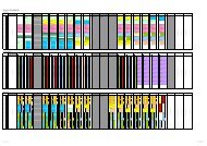
Figure 5. lois <strong>de</strong> comportement <strong>et</strong> spectre é<strong>la</strong>stique<br />
4.2. Dép<strong>la</strong>cements inter-étages:<br />
La contribution <strong>de</strong>s trois premiers mo<strong>de</strong>s est présentée à <strong>la</strong> figure 7.a. Une<br />
comparaison entre les métho<strong>de</strong>s N2, AMP <strong>et</strong> <strong>la</strong> métho<strong>de</strong> temporelle non linéaire<br />
simplifiée a été menée (figure 7.b). L'on peut observer que <strong>de</strong> <strong>la</strong> métho<strong>de</strong> N2<br />
con<strong>du</strong>it à une surestimation <strong>de</strong>s dép<strong>la</strong>cements re<strong>la</strong>tifs inter-étages <strong>de</strong> <strong>la</strong> partie<br />
"supérieure", <strong>et</strong> à une sous-estimation <strong>de</strong> ceux <strong>de</strong> <strong>la</strong> partie "inférieure" par<br />
rapport à l'AMP. Ce<strong>la</strong> est <strong>du</strong> au fait que seul le premier mo<strong>de</strong> est considéré dans<br />
<strong>la</strong> première métho<strong>de</strong>. La métho<strong>de</strong> AMP, donne une