Formation GAUSS AGF â Paris - Thierry Roncalli's Home Page
Formation GAUSS AGF â Paris - Thierry Roncalli's Home Page
Formation GAUSS AGF â Paris - Thierry Roncalli's Home Page

You also want an ePaper? Increase the reach of your titles
YUMPU automatically turns print PDFs into web optimized ePapers that Google loves.
<strong>Formation</strong> <strong>GAUSS</strong><strong>AGF</strong> — <strong>Paris</strong>(Compléments de programmation)<strong>Thierry</strong> RoncalliGroupe de Recherche Opérationnelle du Crédit LyonnaisBercy-Expo — Immeuble Bercy SUD — 4 e étage90, Quai de Bercy — 75613 <strong>Paris</strong> Cedex 12Juin 2003
Table des matièresI NIVEAU I — PRISE EN MAIN DE <strong>GAUSS</strong> 11 Introduction 11.1 Configuration de <strong>GAUSS</strong> . . . . . . . . . . . . . . . . . . . . . . . . . . . . . . . . . . . . . . . . . 11.2 Un premier exemple . . . . . . . . . . . . . . . . . . . . . . . . . . . . . . . . . . . . . . . . . . . 11.3 La philosophie de <strong>GAUSS</strong> . . . . . . . . . . . . . . . . . . . . . . . . . . . . . . . . . . . . . . . . 11.4 L’aide en ligne . . . . . . . . . . . . . . . . . . . . . . . . . . . . . . . . . . . . . . . . . . . . . . 11.5 le debugger . . . . . . . . . . . . . . . . . . . . . . . . . . . . . . . . . . . . . . . . . . . . . . . . 11.6 L’architecture . . . . . . . . . . . . . . . . . . . . . . . . . . . . . . . . . . . . . . . . . . . . . . . 22 Découverte des commandes et des opérateurs de bases 22.1 Déclaration d’une matrice . . . . . . . . . . . . . . . . . . . . . . . . . . . . . . . . . . . . . . . . 22.2 Les opérateurs matriciels . . . . . . . . . . . . . . . . . . . . . . . . . . . . . . . . . . . . . . . . . 22.3 Les sous-matrices . . . . . . . . . . . . . . . . . . . . . . . . . . . . . . . . . . . . . . . . . . . . . 42.4 Les commandes mathématiques . . . . . . . . . . . . . . . . . . . . . . . . . . . . . . . . . . . . . 42.5 Les commandes statistiques . . . . . . . . . . . . . . . . . . . . . . . . . . . . . . . . . . . . . . . 52.6 Les commandes de manipulation de matrices . . . . . . . . . . . . . . . . . . . . . . . . . . . . . 52.7 Les opérateurs conditionnels et relationnels . . . . . . . . . . . . . . . . . . . . . . . . . . . . . . 52.8 Les structures de contrôle . . . . . . . . . . . . . . . . . . . . . . . . . . . . . . . . . . . . . . . . 53 La différence entre une procédure et une commande 54 Quelques explications sur les procédures et les bibliothèques 85 La bibliothèque graphique PGRAPH 165.1 Premier exemple . . . . . . . . . . . . . . . . . . . . . . . . . . . . . . . . . . . . . . . . . . . . . 165.2 Améliorer la mise en forme du graphique . . . . . . . . . . . . . . . . . . . . . . . . . . . . . . . . 175.3 Les fontes graphiques . . . . . . . . . . . . . . . . . . . . . . . . . . . . . . . . . . . . . . . . . . . 185.4 Les légendes . . . . . . . . . . . . . . . . . . . . . . . . . . . . . . . . . . . . . . . . . . . . . . . . 205.5 Le mode fenêtre . . . . . . . . . . . . . . . . . . . . . . . . . . . . . . . . . . . . . . . . . . . . . . 225.5.1 La procédure window . . . . . . . . . . . . . . . . . . . . . . . . . . . . . . . . . . . . . . . 225.5.2 La procédure makewind . . . . . . . . . . . . . . . . . . . . . . . . . . . . . . . . . . . . . 246 Un mot sur les chaînes de caractères 257 La gestion des dates 278 Les entrées et sorties 318.1 La procédure save . . . . . . . . . . . . . . . . . . . . . . . . . . . . . . . . . . . . . . . . . . . . 318.2 Les procédures load, loadf, loadm et loads . . . . . . . . . . . . . . . . . . . . . . . . . . . . . 328.3 Les procédures fopen, f* . . . . . . . . . . . . . . . . . . . . . . . . . . . . . . . . . . . . . . . . 33II NIVEAU II — PROGRAMMATION AVANCÉE <strong>GAUSS</strong> 369 La récursivité 3610 La commande sysstate 3811 Compilation et exécution 41
12 Les directives de compilation 4113 Les procédures 4313.1 Génération de nombre aléatoires gaussiens multidimensionnels . . . . . . . . . . . . . . . . . . . . 4313.2 Une première approche de l’analyse numérique par blocs . . . . . . . . . . . . . . . . . . . . . . . 4414 Les pointeurs 4815 Les variables globales externes 5015.1 La communication des informations entre les procédures d’une même bibliothèque . . . . . . . . 5015.2 La distinction entre les informations indispensables et les informations complémentaires . . . . . 5216 Les bibliothèques 5517 La construction de l’aide en ligne 5818 Inclure des graphiques <strong>GAUSS</strong> dans TeX ou MSWord 6019 Manipulation des variables buffer 6120 Utilisation des commandes varput/varputl et varget/vargetl 6121 La gestion des bases de données 6321.1 Création d’une base de données . . . . . . . . . . . . . . . . . . . . . . . . . . . . . . . . . . . . . 6421.1.1 La procédure saved . . . . . . . . . . . . . . . . . . . . . . . . . . . . . . . . . . . . . . . 6421.1.2 Les commandes create et writer . . . . . . . . . . . . . . . . . . . . . . . . . . . . . . . 6421.2 Visualisation de la base de données . . . . . . . . . . . . . . . . . . . . . . . . . . . . . . . . . . . 6621.3 Manipulation des variables . . . . . . . . . . . . . . . . . . . . . . . . . . . . . . . . . . . . . . . . 6721.4 Lecture des données . . . . . . . . . . . . . . . . . . . . . . . . . . . . . . . . . . . . . . . . . . . 6821.4.1 La procédure loadd . . . . . . . . . . . . . . . . . . . . . . . . . . . . . . . . . . . . . . . 6821.4.2 La commande readr . . . . . . . . . . . . . . . . . . . . . . . . . . . . . . . . . . . . . . . 6921.5 Manipulation et transformation des données . . . . . . . . . . . . . . . . . . . . . . . . . . . . . . 7021.6 Les formats externes . . . . . . . . . . . . . . . . . . . . . . . . . . . . . . . . . . . . . . . . . . . 7221.6.1 Les fichiers ASCII . . . . . . . . . . . . . . . . . . . . . . . . . . . . . . . . . . . . . . . . 7221.6.1.1 Le programme ATOG . . . . . . . . . . . . . . . . . . . . . . . . . . . . . . . . 7221.6.1.2 Les commandes fopen, f* . . . . . . . . . . . . . . . . . . . . . . . . . . . . . . 7221.6.2 Les procédures export/f et import/f . . . . . . . . . . . . . . . . . . . . . . . . . . . . . . 7321.7 Utilisation avancée de l’accès séquentiel . . . . . . . . . . . . . . . . . . . . . . . . . . . . . . . . 7822 L’utilisation des DLLs dans <strong>GAUSS</strong> 81III APPLICATIONS 8323 Optimisation d’une fonction 8323.1 Les procédures optmum et QNewton . . . . . . . . . . . . . . . . . . . . . . . . . . . . . . . . . . . 8323.2 Les procédures co et sqpSolve . . . . . . . . . . . . . . . . . . . . . . . . . . . . . . . . . . . . . 8523.3 La procédure Qprog . . . . . . . . . . . . . . . . . . . . . . . . . . . . . . . . . . . . . . . . . . . 8924 Maximum de vraisemblance 92
25 Méthode des moments généralisés 10125.1 Le principe de la méthode des moments . . . . . . . . . . . . . . . . . . . . . . . . . . . . . . . . 10125.2 L’utilisation des moments simulés . . . . . . . . . . . . . . . . . . . . . . . . . . . . . . . . . . . . 10225.3 La méthode des moments généralisés . . . . . . . . . . . . . . . . . . . . . . . . . . . . . . . . . . 10425.4 Un exemple ARCH . . . . . . . . . . . . . . . . . . . . . . . . . . . . . . . . . . . . . . . . . . . . 10825.5 Les variables instrumentales . . . . . . . . . . . . . . . . . . . . . . . . . . . . . . . . . . . . . . . 11026 Maximum de vraisemblance simulé 11226.1 Calcul de probabilités par simulation . . . . . . . . . . . . . . . . . . . . . . . . . . . . . . . . . . 11226.1.1 Un premier exemple . . . . . . . . . . . . . . . . . . . . . . . . . . . . . . . . . . . . . . . 11226.1.2 Un second exemple . . . . . . . . . . . . . . . . . . . . . . . . . . . . . . . . . . . . . . . . 11426.1.3 Un troisième exemple . . . . . . . . . . . . . . . . . . . . . . . . . . . . . . . . . . . . . . 11426.2 Calcul d’espérances conditionnelles par simulation . . . . . . . . . . . . . . . . . . . . . . . . . . 11826.3 Un exemple simple de maximum de vraisemblance simulé . . . . . . . . . . . . . . . . . . . . . . 11926.4 Le simulateur GHK . . . . . . . . . . . . . . . . . . . . . . . . . . . . . . . . . . . . . . . . . . . . 12027 Données de panel 12227.1 Une petite introduction . . . . . . . . . . . . . . . . . . . . . . . . . . . . . . . . . . . . . . . . . 12227.2 La bibliothèque TSCS . . . . . . . . . . . . . . . . . . . . . . . . . . . . . . . . . . . . . . . . . . 12627.3 Le programme DPD98 de Manuel Arellano et Stephen Bond . . . . . . . . . . . . . . . . . . . . 12827.4 Un programme de Curt Wells . . . . . . . . . . . . . . . . . . . . . . . . . . . . . . . . . . . . . . 13828 Manipulation des bibliothèques disponibles sur Internet 143IV <strong>GAUSS</strong> 4.0 14329 Le debugger 14430 La gestion des bibliothèques 14531 Les générateurs de nombres aléatoires 14832 Les structures 14833 Les nouvelles commandes 150V APPLICATIONS ECONOMETRIQUES 15134 L’analyse en composantes principales 15135 Les méthodes de régression 15535.1 Les moindres carrés ordinaires . . . . . . . . . . . . . . . . . . . . . . . . . . . . . . . . . . . . . . 15735.2 Les moindres carrés non-linéaires . . . . . . . . . . . . . . . . . . . . . . . . . . . . . . . . . . . . 16035.3 Les estimateurs 2SLS et 3SLS . . . . . . . . . . . . . . . . . . . . . . . . . . . . . . . . . . . . . . 16536 Estimation des paramètres d’une équation différentielle stochastique 17436.1 Simulation d’une solution d’équation différentielle stochastique . . . . . . . . . . . . . . . . . . . 17436.2 Estimation par maximum de vraisemblance . . . . . . . . . . . . . . . . . . . . . . . . . . . . . . 17636.3 Estimation par la méthode des moments généralisés . . . . . . . . . . . . . . . . . . . . . . . . . 177
37 Les processus ARCH et GARCH 17937.1 Simulation . . . . . . . . . . . . . . . . . . . . . . . . . . . . . . . . . . . . . . . . . . . . . . . . . 17937.2 Estimation par la méthode du maximum de vraisemblance . . . . . . . . . . . . . . . . . . . . . . 18137.3 Estimation par la méthode des moments généralisés . . . . . . . . . . . . . . . . . . . . . . . . . 18237.4 Prolongements . . . . . . . . . . . . . . . . . . . . . . . . . . . . . . . . . . . . . . . . . . . . . . 18238 Les tests 18238.1 Tests des résidus . . . . . . . . . . . . . . . . . . . . . . . . . . . . . . . . . . . . . . . . . . . . . 18238.1.1 Test de significativité de la régression (linéaire et non-linéaire) . . . . . . . . . . . . . . . 18238.1.2 Test d’autocorrélation des résidus . . . . . . . . . . . . . . . . . . . . . . . . . . . . . . . . 18438.1.3 Test d’observations abérrantes . . . . . . . . . . . . . . . . . . . . . . . . . . . . . . . . . 18638.2 Tests de normalité . . . . . . . . . . . . . . . . . . . . . . . . . . . . . . . . . . . . . . . . . . . . 18638.3 Tests d’hypothèses sur les coefficients . . . . . . . . . . . . . . . . . . . . . . . . . . . . . . . . . . 19039 Intégration et cointégration 19239.1 Tests de racine unité . . . . . . . . . . . . . . . . . . . . . . . . . . . . . . . . . . . . . . . . . . . 19239.1.1 Test KPSS . . . . . . . . . . . . . . . . . . . . . . . . . . . . . . . . . . . . . . . . . . . . 19239.1.2 Test ADF . . . . . . . . . . . . . . . . . . . . . . . . . . . . . . . . . . . . . . . . . . . . . 19639.2 Calcul des valeurs critiques du test ADF par Monte Carlo . . . . . . . . . . . . . . . . . . . . . . 20539.3 Cointégration vectorielle (méthode de Johansen) . . . . . . . . . . . . . . . . . . . . . . . . . . . 20639.3.1 Les procédures . . . . . . . . . . . . . . . . . . . . . . . . . . . . . . . . . . . . . . . . . . 20639.3.2 Détermination du nombre de cointégrations . . . . . . . . . . . . . . . . . . . . . . . . . . 21039.3.3 Estimation du modèle à correction d’erreur vectoriel . . . . . . . . . . . . . . . . . . . . . 21140 Les séries temporelles 212VI <strong>GAUSS</strong> 5.0 21341 Les tableaux multidimensionnels 21342 L’importation et l’exportation de données EXCEL 22243 Un exemple : la gestion de portefeuille 22343.1 Le problème mathématique . . . . . . . . . . . . . . . . . . . . . . . . . . . . . . . . . . . . . . . 22343.2 Un premier exemple . . . . . . . . . . . . . . . . . . . . . . . . . . . . . . . . . . . . . . . . . . . 22543.3 La prise en compte de préférences allocatives et de contraintes techniques . . . . . . . . . . . . . 22744 L’utilisation de Mercury 23044.1 Un premier exemple . . . . . . . . . . . . . . . . . . . . . . . . . . . . . . . . . . . . . . . . . . . 23044.2 Un deuxième exemple . . . . . . . . . . . . . . . . . . . . . . . . . . . . . . . . . . . . . . . . . . 230
1 INTRODUCTIONPremière partieNIVEAU I — PRISE EN MAIN DE <strong>GAUSS</strong>1 Introduction1.1 Configuration de <strong>GAUSS</strong>Le fichier gauss.cfg permet de configurer <strong>GAUSS</strong>. Il est composé de plusieurs parties :– une partie permettant de définir les répertoires (exécutable, bibliothèque, DLLs, bases de données, etc.) ;– une ligne de commande pour spécifier l’éditeur (vi par défaut) ;– une partie pour gérer l’espace de travail ;– et enfin, la déclaration par défaut de certaines variables (qui peuvent être globales).Remarque 1 Nous pouvons généralement changer les valeurs de ces variables localement dans un programmeavec la commande sysstate.1.2 Un premier exempleConsidérons les lignes de commande suivantes :new;x = rndn(100,1);print x;Le mode commande (fenêtre <strong>GAUSS</strong>) permet bien sûr d’exécuter des lignes de commandes, mais il permet ausside récupérer les résultats.– Le fichier gauss.err contient l’ensemble des messages d’erreur d’une session.– Le fichier command.log contient toutes les commandes exécutées. Celui-ci n’est pas initialisé à chaquesession.Exemple 1 Exécutez la commande y = inv(x) qui produit une erreur puisque x est un vecteur.1.3 La philosophie de <strong>GAUSS</strong>– Le concept de langage matriciel (<strong>GAUSS</strong>, MATLAB, etc.)– Les opérateurs E × E– Un langage mathématique=⇒ <strong>GAUSS</strong> n’est pas un logiciel statistique, un logiciel d’économétrie, un logiciel de finance, un logiciel detraitement du signal, etc. Pourtant, <strong>GAUSS</strong> est intensivement utilisé dans chacun de ces domaines. <strong>GAUSS</strong> n’apourtant pas la vocation à devenir par exemple un logiciel de statistiques. Cela reste avant tout un langage deprogrammation mathématique.Remarque 2 La commande stepwise de SAS.1.4 L’aide en lignevoir le supplément Unix.1.5 le debuggervoir le supplément Unix.<strong>Formation</strong> RITME — <strong>Paris</strong>, 1 et 2 Juillet 2003 1
2DÉCOUVERTE DES COMMANDES ET DES OPÉRATEURS DE BASES1.6 L’architecture<strong>GAUSS</strong>HOME| −→ dlib| −→ examples| −→ lib| −→ LServ| −→ src| −→ wksp2 Découverte des commandes et des opérateurs de bases2.1 Déclaration d’une matriceIl existe différentes façons de déclarer une matrice avec la commande let :let x = {1 2,3 4,5 6}; /* Matrice de dimension 3*2 */let x[3,2] = 1 2 3 4 5 6; /* Matrice de dimension 3*2 */let x = 1 2 3 4 5 6; /* Vecteur de dimension 6 */let x[1,6] = 1 2 3 4 5 6; /* Vecteur ligne de dimension 6 */let x = 4; /* scalaire */x = 4; /* scalaire (affectation) */Pour les nombres complexes, on utilise la notation compacte a+bi. Par exemple :let x = {1+5i, 2, 3};Remarque 3 <strong>GAUSS</strong> possède un nouveau scan pour la déclaration des matrices.(voir le fichier readme).2.2 Les opérateurs matricielsOperators, Mathematical and StringOperators====================================== % == eq $== and+ [ .== .eq .$== .and$+ ] >= ge $>= eqv- : .>= .ge .$>= .eqv* , > gt $> not.* . .> .gt .$> .not/ |
2DÉCOUVERTE DES COMMANDES ET DES OPÉRATEURS DE BASES- subtraction or unary minus ~ matrix horizontal concatenation* multiplication $| string array vert concatenation.* ExE multiplication $~ string array horiz concatenation^ ExE exponentiation ’ transpose! factorial .’ bookkeeping transpose./ ExE division/ division or linear equation solution of Ax = b, for example: x = b/A;% modulo division.*. Kronecker product STRING OPERATORS*~ horizontal direct product $+ string concatenationSymbols used for indexing matrices are: ’’[’’, ’’]’’, ’’.’’ and ’’:’’. For example,x[1 2 5] returns the 1st, 2nd and 5th elements of x.x[2:10] returns the 2nd through 10th elements of x.x[.,2 4 6] returns all rows of the 2nd, 4th, and 6th columns of x.x = ones(5,1); /* cre’ation d’un vecteur unitaire */y = zeros(5,2); /* cre’ation d’une matrice nulle */z = eye(5); /* cre’ation d’une matrice identite’ */xz = x * z; /* multiplication */z = 2 + z; /* addition */x = x + x; /* addition */x = x~x; /* concate’nation horizontale */z = z|z: /* concate’nation verticale *//*** Cre’ation de nombres ale’atoires CHI2 10 degre’s de liberte’*/x = rndn(10,4);x = x^2; /* introduction d’un ope’rateur ExE */x = sumc(x);@ ou @x = rndn(10,4);x = x .* x;x = sumc(x);Cette notion d’opérateurs E × E est primordiale pour bien maîtriser <strong>GAUSS</strong>. Considérons le calcul depour x = 1, 2, . . . , 100. Nous avons :f (x) =sin(x) cos(x)x + √ x + 1x = seqa(1,1,100); /* sequence additive */y = (sin(x) .* cos(x)) ./ (x +sqrt(x) + 1); /* f(x) */Calculons maitenant la matrice (f (i) × f (j)) i,j. Nous avons :<strong>Formation</strong> RITME — <strong>Paris</strong>, 1 et 2 Juillet 2003 3
2DÉCOUVERTE DES COMMANDES ET DES OPÉRATEURS DE BASESy = y .* y’;De nouveaux exemples de manipulations E × E :let x[1,2] = 1 2;let y = {3 4,5 6};z = x + y;z = x’ + y;z = x .* y;z = x’ .* y;z = x ./ y;z = y ./ x;z = y ./ x’;2.3 Les sous-matrices– x[r,c] permet d’accéder à l’élément de la r-ième ligne et c-ième colonne.– La syntaxe précédente se généralise lorsque r et c sont des vecteurs.– La notation . permet de sélectionner l’ensemble des lignes/colonnes.– La notation d :f est équivalente à seqa(d,1,d-f+1).x = rndu(150,65);print x[1,1];print x[150,65];print x[1,1]~x[1,2];print x[1,1 2];y = x[1:10 15 25,1 2 5:12 20 21:26];print y;/*** Exemples d’affectation*/y[1,1] = 0;y[1,2] = 1;print y;y[1,1 2] = 0~1;2.4 Les commandes mathématiques– chol : décomposition de Cholesky– det : déterminant d’une matrice– inv : inversion d’une matrice carrée– invpd : inversion d’une matrice pds– eig, eigv, eighv : décomposition vecteurs/valeurs propres– svd : décomposition valeurs sigulières– etc.Exemple 2 (Simulation d’une loi normale multidimensionnelle) Soit Q une matrice telle que Σ =QQ ⊤ , alorsN (µ, Σ) = µ + QN (0, I)<strong>Formation</strong> RITME — <strong>Paris</strong>, 1 et 2 Juillet 2003 4
3 LA DIFFÉRENCE ENTRE UNE PROCÉDURE ET UNE COMMANDEIl existe alors plusieurs décompositions possibles de Σ : La décomposition de Cholesky implique que Q = P, avecla décomposition en valeurs propres Σ = V ΛV ⊤ , nous avons Q = V Λ 1 2 , enfin Q = US 1 2 lorsque nous utilisonsla décomposition en valeurs singulières Σ = USV ⊤ .2.5 Les commandes statistiques– cdf* : fonctions de répartition (par exemple, cdfn)– cdf*c : fonctions de répartition complémentaire (par exemple, cdfnc)– cdf*i : fonctions de répartition inverse ou quantile (par exemple, cdfni)– rnd* : nombres aléatoires (par exemple, rndn)– meanc, stdc, vcx, corrx, quantile, etc.2.6 Les commandes de manipulation de matrices– cols : nombre de colonnes– rows : nombre de lignes– diag : diagonale de la matrice– maxc, minc : maximum & minimum– maxindc, minindc : position des maximum & minimum– miss, missex, missrv, packr : valeurs manquantes– vec, vech, xpnd, reshape, rev : réorganisation des matrices– trimr : élimination des premières et dernières lignes d’une matrice– eye, ones, zeros : matrices identité, unitaire et nulle– imag, real, complex : matrices complexes2.7 Les opérateurs conditionnels et relationnels– Les opérateurs conditionnels : not, and, or, xor et eqv– Les opérateurs conditionnels E × E : .not, .and, .or, .xor et .eqv– Les opérateurs relationnels : eq, ne, gt, lt, ge, le– Les opérateurs relationnels E × E : .eq, .ne, .gt, .lt, .ge, .le– Les opérateurs relationnels (forme symbolique) : ==, /=, >, =, , .=, .
3 LA DIFFÉRENCE ENTRE UNE PROCÉDURE ET UNE COMMANDE(0) : error G0039 : Matrix must be square to invert(gauss) pinv(0|0)Singular values all zeroCurrently active call: PINV [259]Dans l’exemple précédent, nous calculons l’inverse d’un vecteur. Nous obtenons une erreur aussi bien pour lacommande inv que pour la procédure pinv (inverse de Moore-Penrose). Cependant, les messages d’erreurne présentent pas le même format :– Le premier message d’erreur commence par (0) et affiche un code d’erreur <strong>GAUSS</strong> G0039 commençantpar la lettre G.– Le second message d’erreur fait référence à la procédure PINV et affiche un nombre [259].(gauss) x = eye(5)(gauss) y = eye(2)(gauss) x*y(0) : error G0036 : Matrices are not conformable(gauss) crossprd(x,y)C:\<strong>GAUSS</strong>\SRC\CROSSPRD.SRC(41) : error G0058 : Index out of rangeCurrently active call: CROSSPRD [41]Une nouvelle fois, nous obtenons deux formats d’erreur différente. L’explication est la suivante : inv etl’opérateur * sont des commandes intrinsèques de <strong>GAUSS</strong> écrites en langage C ou Fortran, alorsque pinv et crossprd sont des procédures <strong>GAUSS</strong> écrites en langage <strong>GAUSS</strong>. Elles font toutes les deuxparties d’une bibliothèque. D’ailleurs, il est tout à fait possible de visualiser le code, puisque le message d’erreurnous indique dans quel fichier se trouve la procédure correspondante./*** crossprd.src** (C) Copyright 1988-1998 by Aptech Systems, Inc.** All Rights Reserved.**** This Software Product is PROPRIETARY SOURCE CODE OF APTECH** SYSTEMS, INC. This File Header must accompany all files using** any portion, in whole or in part, of this Source Code. In** addition, the right to create such files is strictly limited by** Section 2.A. of the <strong>GAUSS</strong> Applications License Agreement** accompanying this Software Product.**** If you wish to distribute any portion of the proprietary Source** Code, in whole or in part, you must first obtain written** permission from Aptech Systems.****> crossprd**** Purpose: Computes the cross products (vector products) of** sets of 3x1 vectors.**** Format: z = crossprd(x,y);**** Input: x 3xK matrix, each column is treated as a 3x1 vector.**** y 3xK matrix, each column is treated as a 3x1 vector.**<strong>Formation</strong> RITME — <strong>Paris</strong>, 1 et 2 Juillet 2003 6
3 LA DIFFÉRENCE ENTRE UNE PROCÉDURE ET UNE COMMANDE** Output: z 3xK matrix, each column is the cross product** (sometimes called vector product) of the** corresponding columns of x and y.**** Remarks: The cross product vector (z) is orthogonal to both x and y.** sumc(x.*z) and sumc(y.*z) will be Kx1 vectors all of whose** elements are 0 (except for rounding error).**** Globals: None*/proc crossprd(x,y);local r1, r2, r3;r1 = x[2,.].*y[3,.]-x[3,.].*y[2,.];r2 = x[3,.].*y[1,.]-x[1,.].*y[3,.];r3 = x[1,.].*y[2,.]-x[2,.].*y[1,.];retp( r1|r2|r3 );endp;La dernière version de <strong>GAUSS</strong> comprend plus de 800 opérateurs, commandes et procédures. Sur ce nombre, plusde la moitié ne font pas partie du langage <strong>GAUSS</strong>, mais correspondent à la bibliothèque <strong>GAUSS</strong>.Remarque 4 <strong>GAUSS</strong> est un langage relativement puissant, qui permet finalement de tout développer dans celangage. Il existe actuellement une quarantaine de bibliothèques <strong>GAUSS</strong>, et toutes sont écrites en pur langage<strong>GAUSS</strong> sans recourir à d’autres langages tels que le C pour réduire les temps de calcul (politique d’APTECH).– OPTMUM : Bibliothèque d’optimisation (à comparer avec la bibliothèque d’optimisation de S+)– CML & MaxLik : Bibliothèques de maximum de vraisemblance (à comparer avec les procédures équivalentesde SAS).– ARIMA : Procédure d’estimation de modèles ARMA (à comparer avec la procédure de SAS).– TSM : Bibliothèque de séries temporelles (à comparer avec la bibliothèque de signal de MatLab, lesprocédures d’estimation de modèles espace-état de SAS et S+).Les points à développer :1. La notion de procédure2. La notion de bibliothèqueConsidérons la loi de Gumbel. La fonction de distribution correspond à(gauss) x = seqa(-5,0.1,101)(gauss) cdf = exp(-exp(-x))F (x) = exp (− exp (−x))Nous pourrions très bien envisager de créer une fonction (ou une procédure) qui permettrait de calculer F (x)en employant la ligne de commandecdf = cdfGumbel(x) ;La solution est1. Manipulation de la fonction cdfGumbel2. Construction de la bibliothèque ritme(a) Créer un répertoire src/ritmefn cdfGumbel(x) = exp(-exp(-x))(b) Créer un fichier gumbel.src contenant la fonction cdfGumbel<strong>Formation</strong> RITME — <strong>Paris</strong>, 1 et 2 Juillet 2003 7
4 QUELQUES EXPLICATIONS SUR LES PROCÉDURES ET LES BIBLIOTHÈQUES(c) Créer la bibliothèque ritme avec la ligne de commande :lib ritme gumbel.src -a3. Utilisation de la bibliothèque avec la commande :library ritme ;4 Quelques explications sur les procédures et les bibliothèquesLa syntaxe d’une procédure estproc (n) = nom_de_la_procedure(entree_1,entree_2,...,entree_m);local variableLocale_1,variableLocale_2,...,variableLocale_p;local retour_1,retour_2,...,retour_n;/* Code source de la procedure:: Les variables locales servent a definir des calculs intermediaires:: Les variables retour_* sont les variables ’’retour’’ et doivent donc:: etre toujours definies*/retour_1 = ... ;retour_2 = ... ;retour_n = ... ;retp(retour_1,retour_2,...,retour_n);endp;Dans ce cas, l’appel de la procédure se fait de la façon suivante :{retour 1,retour 2 , ...,retour n} =nom de la procedure(entree 1,entree 2,...,entree m) ;Quelques cas particuliers. Si nous désirons excéuter la procédure, mais ne pas définir les retours, nous employonsla commande call :call nom de la procedure(entree 1,entree 2,...,entree m) ;Si le nombre de retour est égal à 1, il n’est pas nécessaire de définir (n). Nous pouvons avoirproc nom de la procedure(entree 1,entree 2,...,entree m) ;Dans ce cas, nous pouvons employer indifférementou plus simplementSi le nombre de retour est égal à zéro, nous avons{retour 1} = nom de la procedure(...) ;retour 1 = nom de la procedure(...) ;proc (0) = nom de la procedure(entree 1,entree 2,...,entree m) ;<strong>Formation</strong> RITME — <strong>Paris</strong>, 1 et 2 Juillet 2003 8
4 QUELQUES EXPLICATIONS SUR LES PROCÉDURES ET LES BIBLIOTHÈQUESNous appelons alors la procédure de la façon suivante :nom de la procedure(entree 1,entree 2,...,entree m) ;Enfin, la syntaxe d’un procédure sans argument d’entrée estproc (n) = nom de la procedure ;Voyons différents exemples :◮ cumsumcproc cumsumc(x);if rows(x) == 1;retp(x);else;retp( recserar(x,x[1,.],ones(1,cols(x)) ) );endif;endp;◮ olsqr2proc (3) = olsqr2(y,x);local flag,n,p,qraux,work,pvt,job,b,k,rsd,xb,info,qy,qty,rd;/* check for complex input */if iscplx(x);if hasimag(x);errorlog ’’ERROR: Not implemented for complex matrices.’’;end;else;x = real(x);endif;endif;if iscplx(y);if hasimag(y);errorlog ’’ERROR: Not implemented for complex matrices.’’;end;else;y = real(y);endif;endif;n = rows(x);p = cols(x);qraux = zeros(p,1);work = qraux;pvt = qraux;flag = 1; /* Use pivoting *//* compute matrix dimensions and other inputs to qrsl subroutine */if rows(y) ne n;errorlog ’’ERROR: OLSQR2 - X and Y must have same length’’;<strong>Formation</strong> RITME — <strong>Paris</strong>, 1 et 2 Juillet 2003 9
4 QUELQUES EXPLICATIONS SUR LES PROCÉDURES ET LES BIBLIOTHÈQUESend;elseif n < p;errorlog ’’ERROR: OLSQR2 - Problem is underdetermined (N < P)’’;end;endif;b = zeros(p,1); /* Vector to hold ols coeffs */rsd = zeros(n,1); /* Vector to hold residuals */xb = rsd; /* Vector to hold predicted values */info = 0;job = 111; /* compute b, rsd, xb */qy = rsd;qty = rsd;k = minc(n|p);x = x’;#ifDLLCALL#else#endifif rows(_qrdc) /= 647 or _qrdc[1] $== 0;_qrdc = zeros(647,1);loadexe _qrdc = qrdc.rex;endif;callexe _qrdc(x,n,n,p,qraux,pvt,work,flag);#ifDLLCALL#endifdllcall qrdc(x,n,n,p,qraux,pvt,work,flag);rd = abs(diag(trimr(x’,0,n-p))); /* abs of diagonal of R */k = sumc( rd .> _olsqtol*rd[1,1] ); /* number of diagonal elements of:: R that are greater than:: tolerance*/#ifDLLCALL#else#endifif rows(_qrsl) /= 455 or _qrsl[1] $== 0;_qrsl = zeros(455,1);loadexe _qrsl = qrsl.rex;endif;callexe _qrsl(x,n,n,k,qraux,y,qy,qty,b,rsd,xb,job,info);<strong>Formation</strong> RITME — <strong>Paris</strong>, 1 et 2 Juillet 2003 10
4 QUELQUES EXPLICATIONS SUR LES PROCÉDURES ET LES BIBLIOTHÈQUES#ifDLLCALL#endifdllcall qrsl(x,n,n,k,qraux,y,qy,qty,b,rsd,xb,job,info);/* sort b to put it in correct order */b = submat( sortc(b~pvt,2),0,1);retp(b,rsd,xb);endp;Les variables locales ne sont pas accesibles en dehors de la procédure. Les variables d’entrée sontaussi des variables locales. Cela veut dire qu’il y a copie des entrées.◮ A titre d’illustration, que fait le programme suivant ?proc f(x);x = x^2;retp(x);endp;x = 2;y = f(x);print y~x;z = f(y);print z~y;Exemple 3 Ecrire une procédure de simulation de nombres χ 2 à n degrés de liberté dont la syntaxe est :u = rndchi(r,c,n) ;Exemple 4 Nous considérons la fonction de distribution “Generalized Extreme Value distribution” (GEV)G (µ, σ, ξ){ [ ( )] − 1}x − µξG (x) = exp − 1 + ξσdéfini sur le support ∆ = { x : 1 + ξ ( ) }x−µσ > 0 . La fonction de densité correspondante estg (x) = 1 [ ( )] −(1+ξ {x − µξ ) [ ( )] − 1}x − µξ1 + ξexp − 1 + ξσ σσLe quantile G −1 (α) d’ordre α pour la distribution GEV est donné par la formule suivante :G −1 (α) = µ − σ [1 − (− ln α) −ξ]ξEcrire quatre procédures pour la fonction de distribution, la fonction de densité, le quantile et la génération denombres aléatoires.◮ Solution proposée :/***> pdfGEV***/<strong>Formation</strong> RITME — <strong>Paris</strong>, 1 et 2 Juillet 2003 11
4 QUELQUES EXPLICATIONS SUR LES PROCÉDURES ET LES BIBLIOTHÈQUESproc pdfGEV(x,mu,sigma,xi);local y,e,pdf;x = (x - mu) ./ sigma;y = (1 + xi .* x);e = y .> 0;y = y .* e + __macheps * (1-e);pdf = (y^(-(1+xi)./xi)) .* exp( -(y^(-1./xi)) ) ./ sigma;pdf = pdf .* e;retp(pdf);endp;/***> cdfGEV***/proc cdfGEV(x,mu,sigma,xi);local y,e,cdf;x = (x - mu) ./ sigma;y = (1 + xi .* x);e = y .> 0;y = y .* e + __macheps * (1-e);cdf = exp(-( y^(-1./xi) ));cdf = cdf .* e + (1-e) .* (xi .< 0);retp(cdf);endp;/***> cdfGEVi***/proc cdfGEVi(alpha,mu,sigma,xi);local cdfi;alpha = miss(miss(alpha,0),1);cdfi = mu - sigma.*(1 - (-ln(alpha))^(-xi))./xi;retp(cdfi);endp;/*<strong>Formation</strong> RITME — <strong>Paris</strong>, 1 et 2 Juillet 2003 12
4 QUELQUES EXPLICATIONS SUR LES PROCÉDURES ET LES BIBLIOTHÈQUES**> rndGEV***/proc rndGEV(r,c,mu,sigma,xi);local u;u = cdfGEVi(rndu(r,c),mu,sigma,xi);retp(u);endp;◮ Manipulation de la procédure OLS (I)/*** ols1.prg***/new;rndseed 123;Nobs = 100;K = 5;sigma = 0.5;x = ones(Nobs,1)~rndu(Nobs,K);beta = seqa(1,1,K+1);y = x*beta + rndn(Nobs,1)*sigma;output file = ols1.out reset;call ols(0,y,x);output off;Valid cases: 100 Dependent variable: YMissing cases: 0 Deletion method: NoneTotal SS: 659.196 Degrees of freedom: 94R-squared: 0.965 Rbar-squared: 0.963Residual SS: 22.988 Std error of est: 0.495F(5,94): 520.297 Probability of F: 0.000Standard Prob Standardized Cor withVariable Estimate Error t-value >|t| Estimate Dep Var-------------------------------------------------------------------------------CONSTANT 0.743400 0.228847 3.248453 0.002 --- ---X1 2.004655 0.191707 10.456887 0.000 0.205635 0.330995X2 3.087867 0.185820 16.617507 0.000 0.322132 0.331370X3 4.307761 0.186731 23.069299 0.000 0.455438 0.314800<strong>Formation</strong> RITME — <strong>Paris</strong>, 1 et 2 Juillet 2003 13
4 QUELQUES EXPLICATIONS SUR LES PROCÉDURES ET LES BIBLIOTHÈQUESX4 5.413424 0.182912 29.595702 0.000 0.589843 0.457336X5 5.665314 0.184540 30.699685 0.000 0.602168 0.626387◮ Manipulation de la procédure OLS (II)/*** ols2.prg***/new;rndseed 123;Nobs = 100;K = 5;sigma = 0.5;x = ones(Nobs,1)~rndu(Nobs,K);beta = seqa(1,1,K+1);y = x*beta + rndn(Nobs,1)*sigma;output file = ols2.out reset;{vnam,m,b,stb,vc,stderr,sigma,cx,rsq,resid,dwstat} = ols(0,y,x);print b;print $vnam;{vnam,vnam,vnam,stb,vc,stderr,sigma,cx,sigma,resid,dwstat} = ols(0,y,x);print $vnam;print sigma;output off;Valid cases: 100 Dependent variable: YMissing cases: 0 Deletion method: NoneTotal SS: 659.196 Degrees of freedom: 94R-squared: 0.965 Rbar-squared: 0.963Residual SS: 22.988 Std error of est: 0.495F(5,94): 520.297 Probability of F: 0.000Standard Prob Standardized Cor withVariable Estimate Error t-value >|t| Estimate Dep Var-------------------------------------------------------------------------------CONSTANT 0.743400 0.228847 3.248453 0.002 --- ---X1 2.004655 0.191707 10.456887 0.000 0.205635 0.330995X2 3.087867 0.185820 16.617507 0.000 0.322132 0.331370X3 4.307761 0.186731 23.069299 0.000 0.455438 0.314800X4 5.413424 0.182912 29.595702 0.000 0.589843 0.457336X5 5.665314 0.184540 30.699685 0.000 0.602168 0.6263870.74339992<strong>Formation</strong> RITME — <strong>Paris</strong>, 1 et 2 Juillet 2003 14
4 QUELQUES EXPLICATIONS SUR LES PROCÉDURES ET LES BIBLIOTHÈQUES2.00465463.08786674.30776095.41342395.6653139X1X2X3X4X5YValid cases: 100 Dependent variable: YMissing cases: 0 Deletion method: NoneTotal SS: 659.196 Degrees of freedom: 94R-squared: 0.965 Rbar-squared: 0.963Residual SS: 22.988 Std error of est: 0.495F(5,94): 520.297 Probability of F: 0.000Standard Prob Standardized Cor withVariable Estimate Error t-value >|t| Estimate Dep Var-------------------------------------------------------------------------------CONSTANT 0.743400 0.228847 3.248453 0.002 --- ---X1 2.004655 0.191707 10.456887 0.000 0.205635 0.330995X2 3.087867 0.185820 16.617507 0.000 0.322132 0.331370X3 4.307761 0.186731 23.069299 0.000 0.455438 0.314800X4 5.413424 0.182912 29.595702 0.000 0.589843 0.457336X5 5.665314 0.184540 30.699685 0.000 0.602168 0.626387X1X2X3X4X5Y0.49452562◮ Manipulation de la procédure OLS (III)/*** ols3.prg***/new;rndseed 123;Nobs = 100;K = 5;sigma = 0.5;x = ones(Nobs,1)~rndu(Nobs,K);<strong>Formation</strong> RITME — <strong>Paris</strong>, 1 et 2 Juillet 2003 15
5 LA BIBLIOTHÈQUE GRAPHIQUE PGRAPHbeta = seqa(1,1,K+1);y = x*beta + rndn(Nobs,1)*sigma;output file = ols3.out reset;__output = 0;{vnam,m,b,stb,vc,stderr,sigma,cx,rsq,resid,dwstat} = ols(0,y,x);print b;__output = 1;let __altnam = C AGE SEXE TAILLE POIDS PAYS NOTE;{vnam,m,b,stb,vc,stderr,sigma,cx,rsq,resid,dwstat} = ols(0,y,x);output off;0.743399922.00465463.08786674.30776095.41342395.6653139Valid cases: 100 Dependent variable: NOTEMissing cases: 0 Deletion method: NoneTotal SS: 659.196 Degrees of freedom: 94R-squared: 0.965 Rbar-squared: 0.963Residual SS: 22.988 Std error of est: 0.495F(5,94): 520.297 Probability of F: 0.000Standard Prob Standardized Cor withVariable Estimate Error t-value >|t| Estimate Dep Var-------------------------------------------------------------------------------C 0.743400 0.228847 3.248453 0.002 --- ---AGE 2.004655 0.191707 10.456887 0.000 0.205635 0.330995SEXE 3.087867 0.185820 16.617507 0.000 0.322132 0.331370TAILLE 4.307761 0.186731 23.069299 0.000 0.455438 0.314800POIDS 5.413424 0.182912 29.595702 0.000 0.589843 0.457336PAYS 5.665314 0.184540 30.699685 0.000 0.602168 0.626387Remarque 5 La procédure OLS est une vieille procédure écrite dans les années 1985. A l’époque, <strong>GAUSS</strong> nepermettait pas les retours multiples. La syntaxe de la procédure était alorsq = ols(dataset,depvar,indvars) ;avec q un buffer matriciel construit avec la procédure vput. Aujourd’hui, une implémentation de la procédureOLS serait différente. Pourquoi ?5 La bibliothèque graphique PGRAPH5.1 Premier exempleNous considérons la fonctionf (x) = sin (x) cos (x) Y (2)3 (x)<strong>Formation</strong> RITME — <strong>Paris</strong>, 1 et 2 Juillet 2003 16
5 LA BIBLIOTHÈQUE GRAPHIQUE PGRAPHDans l’exemple suivant, nous graphons cette fonction. La version UNIX nécessite quelques manipulationsnécessaires afin de déclarer la fenêtre graphique (manipulations qui n’existent pas pour NT).new;library pgraph;proc f(x);local y;y = sin(x) .* cos(x);y = y .* bessely(3,x);retp(y);endp;y = seqa(pi,2*pi/100,301);x = f(y);#IFUNIXlet v = 100 100 640 480 0 0 1 6 15 0 0 2 2;wxy = WinOpenPQG(v,’’XY Plot’’,’’XY’’);call WinSetActive(wxy);#ENDIFxy(y,x);#IFUNIXcall WinSetActive(1);#ENDIF5.2 Améliorer la mise en forme du graphiqueIl existe de nombreuses variables globales pour améliorer la mise en page. Nous pouvons ainsi ajouter untitre, des labels, ajouter une légende, des messages, dessiner des symboles, etc.new;library pgraph;proc f(x);local y;y = sin(x) .* cos(x);y = y .* bessely(3,x);retp(y);endp;y = seqa(pi,2*pi/100,301);<strong>Formation</strong> RITME — <strong>Paris</strong>, 1 et 2 Juillet 2003 17
5 LA BIBLIOTHÈQUE GRAPHIQUE PGRAPHx = f(y);#IFUNIXlet v = 100 100 640 480 0 0 1 6 15 0 0 2 2;wxy = WinOpenPQG(v,’’XY Plot’’,’’XY’’);call WinSetActive(wxy);#ENDIFgraphset;_pdate = ’’ritme ’’;_pnum = 2;title(’’Un exemple de trace’ de fonction’’);xlabel(’’x’’);ylabel(’’f(x)’’);_pcross = 1;_pframe = 0;xy(y,x);#IFUNIXcall WinSetActive(1);#ENDIF5.3 Les fontes graphiquesNous considérons un premier changement de fontes.new;library pgraph;proc f(x);local y;y = sin(x) .* cos(x);y = y .* bessely(3,x);retp(y);endp;y = seqa(pi,2*pi/100,301);x = f(y);#IFUNIXlet v = 100 100 640 480 0 0 1 6 15 0 0 2 2;wxy = WinOpenPQG(v,’’XY Plot’’,’’XY’’);call WinSetActive(wxy);<strong>Formation</strong> RITME — <strong>Paris</strong>, 1 et 2 Juillet 2003 18
5 LA BIBLIOTHÈQUE GRAPHIQUE PGRAPH#ENDIFgraphset;_pdate = ’’ritme ’’;_pnum = 2;fonts(’’complex’’);title(’’Un exemple de trace’ de fonction’’);xlabel(’’x’’);ylabel(’’f(x)’’);_pcross = 1;_pframe = 0;ytics(-0.15,0.15,0.05,5);xtics(pi,7*pi,pi,0);let labx = ’’PI’’ ’’2*PI’’ ’’3*PI’’ ’’4*PI’’ ’’5*PI’’ ’’6*PI’’ ’’7*PI’’;asclabel(labx,0);xy(y,x);#IFUNIXcall WinSetActive(1);#ENDIFVoyons maintenant comment mélanger et appeler plusieurs fontes en même temps.new;library pgraph;proc f(x);local y;y = sin(x) .* cos(x);y = y .* bessely(3,x);retp(y);endp;y = seqa(pi,2*pi/100,301);x = f(y);#IFUNIXlet v = 100 100 640 480 0 0 1 6 15 0 0 2 2;wxy = WinOpenPQG(v,’’XY Plot’’,’’XY’’);call WinSetActive(wxy);#ENDIFgraphset;_pdate = ’’ritme ’’;_pnum = 2;<strong>Formation</strong> RITME — <strong>Paris</strong>, 1 et 2 Juillet 2003 19
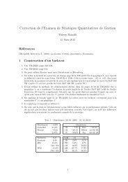
5 LA BIBLIOTHÈQUE GRAPHIQUE PGRAPHfonts(’’complex simgrma’’);title(’’Un exemple de trace’ de fonction\Lf(x) = sin(x) cos(x) Y]3[[(2)](x)’’);xlabel(’’x’’);ylabel(’’\201f(x)’’);_pcross = 1;_pframe = 0;ytics(-0.15,0.15,0.05,5);xtics(pi,7*pi,pi,0);let labx = ’’\202p\201’’ ’’\2012\202p\201’’ ’’\2013\202p\201’’ ’’\2014\202p\201’’’’\2015\202p\201’’ ’’\2016\202p\201’’ ’’\2017\202p\201’’;asclabel(labx,0);graphprt(’’-c=1 -cf=pgraph4.ps’’);xy(y,x);#IFUNIXcall WinSetActive(1);#ENDIFFig. 1 – Un exemple de la bibliothèque PGRAPH5.4 Les légendesnew;library pgraph;<strong>Formation</strong> RITME — <strong>Paris</strong>, 1 et 2 Juillet 2003 20
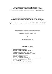
5 LA BIBLIOTHÈQUE GRAPHIQUE PGRAPHproc f(x);local y;y = sin(x) .* cos(x);y = y .* bessely(1~2~3~4,x);retp(y);endp;y = seqa(pi,2*pi/100,301);x = f(y);#IFUNIXlet v = 100 100 640 480 0 0 1 6 15 0 0 2 2;wxy = WinOpenPQG(v,’’XY Plot’’,’’XY’’);call WinSetActive(wxy);#ENDIFgraphset;_pdate = ’’’’;_pnum = 2;fonts(’’complex simgrma’’);title(’’Un exemple de trace’ de fonction\Lf(x) = sin(x) cos(x) Y]\202a\201[[(2)](x)’’);_pltype = 6|1|3|4; _pstype = 8|7|3|5; _plctrl = 0|0|10|10;xlabel(’’x’’);ylabel(’’\201f(x)’’);_pcross = 1;_pframe = 0;ytics(-0.20,0.20,0.05,5);xtics(pi,7*pi,pi,0);let labx = ’’\202p\201’’ ’’\2012\202p\201’’ ’’\2013\202p\201’’ ’’\2014\202p\201’’’’\2015\202p\201’’ ’’\2016\202p\201’’ ’’\2017\202p\201’’;asclabel(labx,0);_plegstr = ’’\202a\201 = 1\000\202a\201 = 2\000\202a\201 = 3\000\202a\201 = 4’’;_plegctl = {2 5 7 0.5};graphprt(’’-c=1 -cf=pgraph5.ps’’);xy(y,x);#IFUNIXcall WinSetActive(1);#ENDIF<strong>Formation</strong> RITME — <strong>Paris</strong>, 1 et 2 Juillet 2003 21
5 LA BIBLIOTHÈQUE GRAPHIQUE PGRAPHFig. 2 – Un second exemple de la bibliothèque PGRAPH5.5 Le mode fenêtreIl est possible d’afficher plusieurs graphes simultanément. Pour cela, nous utilisons le mode fenêtre. Lescommandes de base sont– begwind : initialisation du mode fenêtre– window : construction de fenêtres proportionnelles– makewind : construction de fenêtres non proportionnelles– setwind : sélection d’une fenêtre– endwind : termine le mode fenêtre5.5.1 La procédure windowNous considérons le problème de programmation linéaire suivant :max f (x) = 14x 1 + αx 2 + 13x 3avec/*** Qprog1.prg***/⎧⎨⎩x 1 + x 2 + x 3 ≤ 406x 1 + 9x 2 + 5x 3 ≤ 280x i ≥ 0new;<strong>Formation</strong> RITME — <strong>Paris</strong>, 1 et 2 Juillet 2003 22
5 LA BIBLIOTHÈQUE GRAPHIQUE PGRAPHlibrary pgraph;alpha = seqa(5,0.1,251);N = rows(alpha);x = zeros(N,3);fmax = zeros(N,1);let bounds = {0 1e200};let C[2,3] = 1 1 1 6 9 5;let D = 40 280;sv = ones(3,1)/3;i = 1;do until i > rows(alpha);r = 14|alpha[i]|13;{xi,u1,u2,u3,u4,retcode} = QProg(sv,zeros(3,3),r,0,0,-C,-D,bounds);x[i,.] = xi’;fmax[i] = r’xi;i = i + 1;endo;#IFUNIXlet v = 100 100 640 480 0 0 1 6 15 0 0 2 2;wxy = WinOpenPQG(v,’’XY Plot’’,’’XY’’);call WinSetActive(wxy);#ENDIFgraphset;begwind;window(2,2,0);_pnum = 2; _paxht = 0.25; _pnumht = 0.25;fonts(’’simplex simgrma’’);setwind(1);_pltype = 6|1|3; _pcolor = 3|6|2;xtics(5,30,5,5);ytics(-10,50,10,2);xlabel(’’\202a\201’’);xy(alpha,x);setwind(2);ylabel(’’x]1[(\202a\201)’’);_plctrl = -10; _pstype = 5;xy(alpha,x[.,1]);setwind(3);ylabel(’’x]2[(\202a\201)’’);<strong>Formation</strong> RITME — <strong>Paris</strong>, 1 et 2 Juillet 2003 23
5 LA BIBLIOTHÈQUE GRAPHIQUE PGRAPH_plctrl = 50; _pstype = 9;xy(alpha,x[.,2]);setwind(4);ylabel(’’x]3[(\202a\201)’’);_plctrl = -10; _psymsiz = 6;_pmsgstr = ’’Ici, les symboles sont\000plus grands’’;_pmsgctl = -10~50~0.45~-40~1~13~0 |10~-5~0.25~0~1~12~0 ;xy(alpha,x[.,3]);graphprt(’’-c=1 -cf=qprog1.ps’’);endwind;#IFUNIXcall WinSetActive(1);#ENDIFFig. 3 – Le mode multi-fenêtres5.5.2 La procédure makewindvoir l’exemple de la formation CCF (page 42).<strong>Formation</strong> RITME — <strong>Paris</strong>, 1 et 2 Juillet 2003 24
6 UN MOT SUR LES CHAÎNES DE CARACTÈRES6 Un mot sur les chaînes de caractères◮ Manipulation I : initialiser une chaîne de caractères/*** string1.prg*/new;output file = string1.out reset;str = ’’Il fait beau aujourd’hui’’;print str;l = strlen(str);print l;str1 = strsect(str,1,7);print str1;str = str $+ ’’\L’’ $+ str $+ ’’\t’’ $+ str;print str;output off;Il fait beau aujourd’hui24.000000Il faitIl fait beau aujourd’huiIl fait beau aujourd’hui Il fait beau aujourd’hui◮ Manipulation II : la commande ftos/*** string2.prg*/new;output file = string1.out on;str = ’’Il fait beau aujourd’hui’’;l = strlen(str);str1 = ’’La longueur de la chaine de caracteres \34’’ $+ str $+ ’’\34 est egale a’’;str1 = str1 $+ ftos(l,’’ %lf caracteres.’’,4,3);print str1;output off;La longueur de la chaine de caracteres ’’Il fait beau aujourd’hui’’ est egale a 24.000 caracteres.<strong>Formation</strong> RITME — <strong>Paris</strong>, 1 et 2 Juillet 2003 25
6 UN MOT SUR LES CHAÎNES DE CARACTÈRES◮ Manipulation III : la différence avec un vecteur de caractères/*** string3.prg*/new;outwidth 256;output file = string3.out reset;let x = ’’Janvier’’ ’’Fevrier’’ ’’Mars’’ ’’Avril’’;print x;print $x;let x = Janvier Fevrier Mars Avril;print $x;y = x $+ x;print $y;y = ’’’’ $+ x $+ x;print y;y = reshape(y,3,5);print y;output off;1.6373109e-3061.6373108e-3069.5694382e-3152.3004960e-312JanvierFevrierMarsAvrilJANVIERFeVRIERMARSAVRILJANVIERJFeVRIERFMARSMARSAVRILAVRJANVIERJANVIER<strong>Formation</strong> RITME — <strong>Paris</strong>, 1 et 2 Juillet 2003 26
7 LA GESTION DES DATESFeVRIERFeVRIERMARSMARSAVRILAVRILJANVIERJANVIER FeVRIERFeVRIER MARSMARS AVRILAVRIL JANVIERJANVIERFeVRIERFeVRIER MARSMARS AVRILAVRIL JANVIERJANVIER FeVRIERFeVRIERMARSMARS AVRILAVRIL JANVIERJANVIER FeVRIERFeVRIER MARSMARS◮ Manipulation IV : les tableaux de chaînes de caractères/*** string4.prg*/new;output file = string4.out reset;sa = ’’’’ $+ zeros(500,4);sa[250,3] = ’’<strong>Formation</strong> ritme’’;let string sa[2,3] = ’’pentium’’ ’’intel’’ ’’unix’’ ’’NT’’ ’’PC’’ ’’Gauss’’;print sa;sa = sa $~(sa[.,3] $+ ’’-’’ $+ sa[.,3]);print sa;print (sa .$== ’’unix’’);output off;pentium intel unixNT PC Gausspentium intel unix unix-unixNT PC Gauss Gauss-Gauss0.00000000 0.00000000 1.0000000 0.000000000.00000000 0.00000000 0.00000000 0.000000007 La gestion des dates<strong>GAUSS</strong> possède différentes commandes pour gérer les dates :Time and Date Functions----------------------------------------------------------------------------date Returns current date as { yy,mm,dd,ss }.datestrReturns current date as mm/dd/yy string.dayinyrReturns day number of current date.<strong>Formation</strong> RITME — <strong>Paris</strong>, 1 et 2 Juillet 2003 27
7 LA GESTION DES DATESetdaysethsecetstrComputes difference between two times (days).Computes difference between two times (hsecs).Converts elapsed time to string.hsecElapsed time since midnight, in hsecs.timeReturns current system time.timestrFormats time as hh:mm:ss string.----------------------------------------------------------------------------Use hsec to time segments of code. For example,et = hsec;x = y*y;et = hsec - et;will time the multiplication operator.Year 2000 Considerations------------------------<strong>GAUSS</strong> for Unix 3.2.38 has been certified as Year 2000-ready.However, since <strong>GAUSS</strong> is a programming language, it is entirely possible forthe user to introduce data into a program that is not Year 2000-compliant,particularly when specifying date information.<strong>GAUSS</strong> provides various functions to manipulate dates as set forthbelow. TO ENSURE CORRECT RESULTS, 4 DIGIT YEAR DATA MUST BE USED.Date FunctionPurpose====================================================================d = date;returns current date in a 4-element column vectord = datestr(d); formats date as a string: mo/dy/yrd = datestrymd(d); formats date as a string: yyyymmddd = datestring(d); formats date as a string: mo/dy/yyyyetdy = etdays(ds,de); elapsed time between dates in dayseths = ethsec(ds,de); elapsed time between dates in 100th’s of secondsdaynum = dayinyr(dt); day number in year of a datea. Function datestr(d): datestr(d) formats a date using only the lasttwo digits of the year. Since a date formatted using only two digits forthe year results in a loss of information, it is up to the user toguarantee that dates so formatted are not misused leading to incorrectprogram results. This applies also to date information that is exported toor imported from other programs.datestr is provided *only* for backwards compatibility with legacy programs.b. Sysstate Base Year Toggle: In early versions of <strong>GAUSS</strong> for Unix andWindows, the date function returned (in the year element) the number ofyears since 1900 instead of the actual 4 digit year. This has been fixedand <strong>GAUSS</strong> now returns the actual 4 digit year. However, a Sysstate Optionhas been added to provide users backwards compatibility with code that may<strong>Formation</strong> RITME — <strong>Paris</strong>, 1 et 2 Juillet 2003 28
7 LA GESTION DES DATEShave been written with these earlier versions. (See Sysstate, Case 30, BaseYear Toggle). If you have programs that assume the year element containsthe number of years since 1900, we recommend that you modify your code touse the actual 4 digit year. In the interim, you may use the Sysstate BaseYear Toggle so that your programs will run as expected.Voici quelques exemples de manipulation de dates :new;output file = date1.out reset;d0 = {2000,01,01,0};d = date;et = etdays(d,d0);print et;print dayinyr(d);print datestr(d);print datestrymd(d);print datestring(d);et = ethsec(d,d0);print etstr(et);output off;101.00000265.000009/22/99199909229/22/1999100 days 12 hours 33 minutes 4.92 secondsDans l’exemple suivant, nous illustrons l’utilisation de la commande sysstate.new;output file = date2.out reset;oldsysdate = sysstate(30,1);d = date;print datestring(d);oldsysdate = sysstate(30,0);d = date;print datestring(d);call sysstate(30,oldsysdate);d = date;print datestring(d);<strong>Formation</strong> RITME — <strong>Paris</strong>, 1 et 2 Juillet 2003 29
7 LA GESTION DES DATESoutput off;9/22/19999/22/00999/22/1999Pour mesurer les temps de calcul, nous utilisons les commandes hsec ou ethsec. Voyons un premier exemple.new;cls;t0 = hsec;x = rndn(300,300);x = invpd(x’x);t1 = hsec;output file = date3.out reset;print ftos(t1-t0,’’Temps de calcul : %lf centie‘mes de secondes’’,4,2);print ftos(t1-t0,’’Temps de calcul : %*.*lf centie‘mes de secondes’’,4,2);print ftos(t1-t0,’’Temps de calcul : %*.*lE centie‘mes de secondes’’,4,2);print ftos(t1-t0,’’Temps de calcul : %#*.*lG centie‘mes de secondes’’,4,2);print ftos(t1-t0,’’Temps de calcul : %*.*lG centie‘mes de secondes’’,4,2);print ftos(t1-t0,’’Temps de calcul : %- *.*lf centie‘mes de secondes’’,4,2);print ftos(t1-t0,’’Temps de calcul : %- *.*lE centie‘mes de secondes’’,4,2);print ftos(t1-t0,’’Temps de calcul : %- #*.*lG centie‘mes de secondes’’,4,2);print ftos(t1-t0,’’Temps de calcul : %- *.*lG centie‘mes de secondes’’,4,2);print (t1-t0)/100;format /rd 18,6;print (t1-t0)/100;t = t1-t0;print etstr(t);print etstr(5600);print etstr(256250);print etstr(125256250);print etstr(10125256250);output off;format /mat /on /mb1 /ros 16,8;format /sa /on /mb1 /ros 16,-1;format /str /off /mb1 /ros 16,-1;Temps de calcul : 263.00 centie‘mes de secondesTemps de calcul : 263.00 centie‘mes de secondesTemps de calcul : 2.63E+002 centie‘mes de secondesTemps de calcul : 2.6E+002 centie‘mes de secondes<strong>Formation</strong> RITME — <strong>Paris</strong>, 1 et 2 Juillet 2003 30
8 LES ENTRÉES ET SORTIESTemps de calcul : 2.6E+002 centie‘mes de secondesTemps de calcul : 263.00 centie‘mes de secondesTemps de calcul : 2.63E+002 centie‘mes de secondesTemps de calcul : 2.6E+002 centie‘mes de secondesTemps de calcul : 2.6E+002 centie‘mes de secondes2.63000002.6300002.63 seconds56.00 seconds42 minutes 42.50 seconds14 days 11 hours 56 minutes 2.50 seconds1171 days 21 hours 42 minutes 42.50 seconds8 Les entrées et sorties8.1 La procédure saveSyntaxe :Purpose:Saves symbols to a disk file.Format: save [path = dpath] x, [lpath = ] y;Input: dpath literal or ^string, the default path to use for thisand all subsequent save commands, until changed byanother path = subcommand.x the symbol to be saved. The file will have the samename as the symbol, with the proper extension for thattype of symbol added.lpath literal or ^string, a local path and filename to beused for a particular symbol. The path overrides anydefault path and the filename overrides the name ofthe object. The extension cannot be overridden.save can be used to save matrices, strings or string arrays, procedures,functions and keywords. Procedures, functions and keywords must be compiled andresident in memory before they can be save’d. The file extensions given fordifferent symbol types are:procedure .fcg matrix .fmtfunction .fcg string .fstkeyword .fcg string array .fstLa commande save permet donc de sauvegarder différents types de données (matrices ou tableaux de chaînesde caractères).new;x = rndn(10,10);/* Cre’ation d’un fichier x.fmt */save x;/* Cre’ation d’un fichier avec un nom plus complexe */save un-fichier-contenant-des-nombres-aleatoires = x;<strong>Formation</strong> RITME — <strong>Paris</strong>, 1 et 2 Juillet 2003 31
8 LES ENTRÉES ET SORTIES/* Cre’ation d’un fichier avec un nom plus complexe */save un-fichier-contenant-des-nombres-aleatoires = x;x = ’’une chaine de caracteres’’;save un-fichier-contenant-une-chaine-de-caracteres = x;let string x[1,2] = ’’une chaine de caracteres’’ ’’une deuxieme chaine de caracteres’’;save un-fichier-contenant-un-tableau-de-chaines-de-caracteres = x;output file = save.out reset;fnames = filesa(’’*.f*’’);print fnames;output off;UN-FICHIER-CONTENANT-DES-NOMBRES-ALEATOIRES.fmtUN-FICHIER-CONTENANT-UN-TABLEAU-DE-CHAINES-DE-CARACTERES.FSTUN-FICHIER-CONTENANT-UNE-CHAINE-DE-CARACTERES.FSTX.fmt8.2 Les procédures load, loadf, loadm et loads◮ Chargement d’une matrice (.fmt)new;output file = load1.out reset;x = rndn(5,1);save x;save y = x;load y;load nom_de_variable = x;print x~y~nom_de_variable;output off;-0.95877623 -0.95877623 -0.958776231.0390460 1.0390460 1.0390460-0.36588347 -0.36588347 -0.36588347-0.83261601 -0.83261601 -0.832616011.5656592 1.5656592 1.5656592◮ Chargement d’une chaîne de caractères (.fst)(gauss) xx = ’’une chaine de caracteres’’;(gauss) save xx; /* x.fst */(gauss) load xx; /* xx.fmt */C:\<strong>GAUSS</strong>\ritme\LOAD2.PRG(7) : error G0014 : ’XX.FMT’ : File not<strong>Formation</strong> RITME — <strong>Paris</strong>, 1 et 2 Juillet 2003 32
8 LES ENTRÉES ET SORTIESfound (gauss) load xx.fst;load XX.FST^C:\<strong>GAUSS</strong>\ritme\LOAD3.PRG(5) : error G0008 : ’.FST’ : Syntax error1 error(s)(gauss) load xx = xx.fst(gauss) loads xx8.3 Les procédures fopen, f*– fopen : ouverture d’un fichier (mode ascii ou binaire)– close : fermeture d’un fichier– eof : teste la fin d’un fichier– fgets, fgetsa, fgetsat, fgetst : lecture des données– fputs, fputst : écriture d’un fichier– fseek : positionne le pointeur– ftell : position du pointeur– fcheckerr, fclearerr, fflush, fstrerror◮ Premier exemple :/*** fopen*/new;output file = fopen.out reset;let string x[2,1] = ’’Il fait beau’’ ’’Il ne fait pas beau’’;fw = fopen(’’un_simple_essai’’,’’w’’); /* ouverture en mode e’criture */i = 1;do until i > 250;call fputs(fw,x);i = i + 1;endo;str = getf(’’un_simple_essai’’,0);print strsect(str,1,50);let string x[2,1] = ’’Il fait beau\L’’ ’’Il ne fait pas beau\L’’;fw = fopen(’’un_simple_essai’’,’’w’’); /* ouverture en mode e’criture */i = 1;do until i > 250;call fputs(fw,x);i = i + 1;endo;<strong>Formation</strong> RITME — <strong>Paris</strong>, 1 et 2 Juillet 2003 33
8 LES ENTRÉES ET SORTIESstr = getf(’’un_simple_essai’’,0);print strsect(str,1,50);output off;Il fait beauIl ne fait pas beauIl fait beauIl ne fIl fait beauIl ne fait pas beauIl fait beauI◮ Deuxième exemple :/*** fseek*/new;output file = fseek.out reset;fr = fopen(’’un_simple_essai’’,’’r’’); /* ouverture en mode lecture */pos = ftell(fr);print pos;str1 = fgets(fr,50);print str1;print strlen(str1);pos = ftell(fr);print pos;str2 = fgets(fr,50);print str2;print strlen(str2);pos = ftell(fr);print pos;str3 = fgets(fr,50);print str3;print strlen(str3);pos = ftell(fr);print pos;print strlen(str1)+strlen(str2)+strlen(str3);closeall;output off;0.00000000Il fait beau<strong>Formation</strong> RITME — <strong>Paris</strong>, 1 et 2 Juillet 2003 34
8 LES ENTRÉES ET SORTIES13.00000014.000000Il ne fait pas beau20.00000035.000000Il fait beau13.00000049.00000046.000000<strong>Formation</strong> RITME — <strong>Paris</strong>, 1 et 2 Juillet 2003 35
9 LA RÉCURSIVITÉDeuxième partieNIVEAU II — PROGRAMMATIONAVANCÉE <strong>GAUSS</strong>9 La récursivitéCette notion est très importante. Pourtant, elle n’est documentée nulle part et beaucoup d’utilisateurs <strong>GAUSS</strong>ne sont pas informés de l’existence de cette possibilité. Pour bien comprendre la récursivité, nous considéronsl’exemple de la factorielle. Nous avonsn! = n × (n − 1)!avec 1! = 1. En notant f (n) = n!, nous avons alors une fonction de récurrence. Celle-ci peut être facilementimplémentée dans <strong>GAUSS</strong> et nous vérifions bien que la procédure factorial donne le même résultat quel’opérateur !.new;proc factorial(n);if n > 1;retp(n*factorial(n-1));else;retp(1);endif;endp;output file = recurs1.out reset;factorial(5);print 5!;output off;120.0000120.0000Remarque 6 Attention, la mise en place de la récursivité en informatique n’est pas toujours très naturelle etne correspond pas forcément à la logique humaine. En effet, la structure de la procédure pourrait nous fairepenser que n prend les valeurs successives 5, 4, 3, 2 et enfin 1. Or, cela fonctionne à l’envers. Pourquoi ? Toutsimplement parce que nous pouvons calculer f (n) à partir de f (n − 1) mais non le contraire.new;proc factorial(n);local y;if n > 1;y = n*factorial(n-1);else;y = 1;<strong>Formation</strong> RITME — <strong>Paris</strong>, 1 et 2 Juillet 2003 36
9 LA RÉCURSIVITÉendif;print n~y;retp(y);endp;output file = recurs2.out reset;call factorial(5);output off;1.0000 1.00002.0000 2.00003.0000 6.00004.0000 24.00005.0000 120.0000La propriété de récursivité est particulièrement utile pour la construction des arbres (notament en finance).Considérons par exemple la fonction suivantef 1 (x) =1p1 + x + (1 − p) 11 − xf 2 (x) =1p1 + p 11+x + (1 − p) 11−x+ (1 − p)f 3 (x) = . . .11 − p 11+x − (1 − p) 11−xLe programme suivant illustre comment nous utilisons la récursivité pour calculer f n (x).new;proc tree(x,n,p);local y;if n > 1;y = p ./ (1+tree(x,n-1,p)) + (1-p) ./ (1-tree(x,n-1,p));else;y = p ./ (1+x) + (1-p) ./ (1-x);endif;retp(y);endp;output file = recurs2.out reset;tree(5,1,0.25);n = 1;x = 5;p = 0.25;y = p ./ (1+x) + (1-p) ./ (1-x);<strong>Formation</strong> RITME — <strong>Paris</strong>, 1 et 2 Juillet 2003 37
10 LA COMMANDE SYSSTATEprint y;tree(5,2,0.25);n = 2;x = 5;p = 0.25;y = p ./ ( 1 + p ./ (1+x) + (1-p) ./ (1-x) )+ (1-p) ./ (1 - p ./ (1+x) - (1-p) ./ (1-x) );print y;output off;-0.1458-0.14580.94720.9472Il faut savoir que la récursivité est généralement gourmante en temps de calcul. Elle peut aussi être une solutioninadaptée, surtout lorsque nous sommes aussi intéressés par les valeurs intermédiaires prises par la fonction.Néanmoins, elle permet dans certains cas d’écrire un code élégant et d’exploiter de plus les fonctionnalités desopérateurs E × E de <strong>GAUSS</strong>.new;library pgraph;proc tree(x,n,p);local y;if n > 1;y = p ./ (1+tree(x,n-1,p)) + (1-p) ./ (1-tree(x,n-1,p));else;y = p ./ (1+x) + (1-p) ./ (1-x);endif;retp(y);endp;x = seqa(-5,.1,101);p = seqa(0,0.1,11)’;y = tree(x,10,p);Remarque 7 La procédure sortmc de <strong>GAUSS</strong> exploite la propriété de récursivité pour effectuer un tri multicolonnes.10 La commande sysstateCette commande permet d’obtenir les valeurs des paramètres système et de les modifier. La syntaxe généraleest :{rets...} = sysstate(case,x) ;L’argument case peut prendre différentes valeurs :<strong>Formation</strong> RITME — <strong>Paris</strong>, 1 et 2 Juillet 2003 38
10 LA COMMANDE SYSSTATE1 Version Information2 EXE file location3 loadexe path4 <strong>GAUSS</strong> System Paths save path5 load, loadm path6 loadf, loadp path7 loads path8 Complex Number Toggle9 Complex Trailing Character10 Printer Width11 Auxiliary Output Width12 Precision13 Lu Tolerance14 Cholesky Tolerance15 Screen State16 Automatic print Mode17 Automatic lprint Mode18 Auxiliary Output19 print Format21 Imaginary Tolerance22 Source Path24 Dynamic Library Directory27 Missings Comparison Toggle30 Base Year ToggleCette commande est peu utilisée dans la pratique, pourtant elle se révèle très importante. Voyons quelquesexemples pratiques d’application. Nous cherchons à créer un fichier temporaire dans lequel nous voulons stockercertaines informations. Une première solution peut être la suivante :screen off;outwidth 256;TempFile = tempname(0,0,0);output file = ^TempFile reset;/***> Affichage de rsultats intermdiaires dans un fichier temporaire***/print ’’Affichage de rsultats intermdiaires dans un fichier temporaire’’;output off;Dans un premier temps, nous supprimons l’affichage à l’écran. Ensuite, nous modifions la largeur de la sortieauxiliaire. Enfin, nous créons un fichier temporaire et stockons les informations dans ce fichier. Le problème ducode précédent est de modifier de façon définitive (et non temporaire) les paramètres système. C’est pourquoile code suivant est plus approprié :oldwidth = sysstate(11,0);<strong>Formation</strong> RITME — <strong>Paris</strong>, 1 et 2 Juillet 2003 39
10 LA COMMANDE SYSSTATEcall sysstate(11,256);{oldstate,oldfile} = sysstate(18,0);if oldstate;output off;endif;oldscreen = sysstate(15,0);screen off;TempFile = tempname(0,0,0);output file = ^TempFile reset;/***> Affichage de rsultats intermdiaires dans un fichier temporaire***/print ’’Affichage de rsultats intermdiaires dans un fichier temporaire’’;output off;output file = ^oldfile;if oldstate;output on;else;output off;endif;call sysstate(11,oldwidth);if oldscreen;screen on;endif;Dans ce cas, la sortie auxiliare n’est pas interompue et le système est remis dans son état d’origine (aspect del’écran, largeur de la sortie auxiliaire, etc.).Nous pouvons connaître l’emplacement du programme gauss.exe avec l’instructionsysstate(2,0) ;Voici un exemple d’utilisation de sysstate(1,0) qui peut parfois se révéler très utile :proc sysstate1(args);local vi,version;vi = sysstate(1,0);version = 1000*vi[1] + 100*vi[2] + vi[3]; /* 3.2.35 ===> version = 3235 */if version > 3200;<strong>Formation</strong> RITME — <strong>Paris</strong>, 1 et 2 Juillet 2003 40
12 LES DIRECTIVES DE COMPILATION/* algorithme utilisant les fonctions de <strong>GAUSS</strong> ver. > 3.2.20 */else;/* algorithme n’utilisant pas ces fonctions */endif;retp(rets);endp;11 Compilation et exécution Pour exécuter un programme, nous utilisons la commande run :run nom du programmeCette commande permet en fait de compiler dans un premier temps le programme et dans un deuxièmetemps d’interpréter le pseudo-code. Elle est donc équivalente àcompile programme.prg ;run programme.gcg ; La compilation au préalable d’un programme est vraiment intéressante, si celui-ci est important et sile programme est souvent utilisé. Dans ce cas, nous pouvons charger le code compilé dans un autreprogramme avec la commande use. Notons aussi que la commande saveall permet de sauvergarder la table de symbole de <strong>GAUSS</strong>, qui peutêtre rechargée avec la commande use. Pour exécuter des programmes en mode batch, nous devons fermer la session <strong>GAUSS</strong> en cours à partirdu programme lui-même. Il faut alors utiliser la commande system.12 Les directives de compilationL’utilisation des directives de compilation est particulière. Elles permettent surtout de développer des bibliothèquescompatibles pour différentes plateformes et de prendre en compte les caractéristiques de chaquesystème d’exploitation. Voyons un premier exemple avec la directive de compilation #define :new;#define e 2.7182818print e;x = e + e;print x;show;2.71828185.4365636<strong>Formation</strong> RITME — <strong>Paris</strong>, 1 et 2 Juillet 2003 41
12 LES DIRECTIVES DE COMPILATIONX8 bytes at [01c40020] 1,1 MATRIX65536 bytes program space, 0% used62849008 bytes workspace, 62849000 bytes free1 global symbols, 1500 maximum, 1 shownCet exemple montre que le symbole e est une autre écriture de la valeur numérique 2.7182818. Mais ce n’estpas une variable (elle ne fait pas partie de la table des symboles).Les directives de compilation s’avèrent finalement indispensables pour l’élaboration d’une bibliothèque multiplateforme.Les bibliothèques d’Aptech, comme la bibliothèque intrinsèque <strong>GAUSS</strong>, les utilise fréquement, cequi permet d’utiliser le même code source pour la version Windows et pour la version Unix.#ifUNIXprint ’’systme Unix’’;#elseprint ’’autre systme’’;#endif#ifDOSprint ’’systme Dos’’;#elseprint ’’autre systme’’;#endif#ifOS2WINprint ’’systme Os2-Windows’’;#elseprint ’’autre systme’’;#endif#ifDLLCALLprint ’’systme supportant les DLLs’’;#elseprint ’’systme ne supportant pas les DLLs’’;#endif#ifLIGHTprint ’’version Light de <strong>GAUSS</strong>’’;#elseprint ’’version professionnelle de <strong>GAUSS</strong>’’;#endif#ifREALprint ’’version <strong>GAUSS</strong>-386’’;#elseprint ’’version <strong>GAUSS</strong>-386i’’;<strong>Formation</strong> RITME — <strong>Paris</strong>, 1 et 2 Juillet 2003 42
13 LES PROCÉDURES#endif#ifCPLXprint ’’version <strong>GAUSS</strong>-386i’’;#elseprint ’’version <strong>GAUSS</strong>-386’’;#endifRemark 1 Il existe aussi une directive de compilation #include qui permet d’inclure dans un programme unautre fichier source. Ceci est notamment très utile lorsque plusieurs programmes possèdent une partie commune.13 Les procédures13.1 Génération de nombre aléatoires gaussiens multidimensionnelsNous considérons la construction d’une procédure de génération de nombre aléatoires gaussiens multidimensionnelsbasée sur l’algorithme de Cholesky. La procédure rndmn est classique, mais présente un doubleintérêt :1. La procédure teste si la matrice de covariance est PD. Pour cela, nous autorisons la décomposition deCholesky même si la matrice n’est pas PD avec la commande trap 1,1 ; puis nous testons si une erreurest survenue avec la commande scalerr.2. Si la matrice n’est pas PD, nous affichons un message d’erreur avec la commande errorlog et nousrenvoyons un message d’erreur qui correspond ici à une valeur manquante.Remarque 8 Pourquoi ne pas utiliser la commande print à la place de la commande errorlog ?Nous allons utiliser l’exemple numérique plusieurs fois. Pour cela, nous créons un fichier contenant les donnéesdu problème qui sera appelée avec la directive de compilation #include.La procédureproc (1) = rndmn(mu,SIGMA,N);local K,u,Pchol,y;local oldtrap;K = rows(mu);u = rndn(K,N);oldtrap = trapchk(1);trap 1,1;Pchol = chol(SIGMA)’;trap oldtrap,1;if scalerr(Pchol);ERRORLOG ’’erreur: SIGMA n’est pas une matrice PD.’’;retp(error(0));endif;y = mu + Pchol*u;retp(y’);endp;Le fichier rndmn.inc<strong>Formation</strong> RITME — <strong>Paris</strong>, 1 et 2 Juillet 2003 43
13 LES PROCÉDURESlet sigma[3,3] = 3 0.25 0.50.25 5 -0.90.5 -0.9 2;mu = 10|15|17;L’exemplenew; library ritme;#include rndmn.inc;y = rndmn(mu,SIGMA,1000);output file = rndmn1.out reset;print ’’mu = ’’ mu;print ’’estimation = ’’ meanc(y);print;print ’’SIGMA = ’’ SIGMA;print ’’estimation = ’’ vcx(y);output off;mu =10.00000015.00000017.000000estimation =10.04647615.06275317.082670SIGMA =3.0000000 0.25000000 0.500000000.25000000 5.0000000 -0.900000000.50000000 -0.90000000 2.0000000estimation =3.0379946 0.22053032 0.614005500.22053032 5.0675993 -0.910231700.61400550 -0.91023170 2.159271013.2 Une première approche de l’analyse numérique par blocs<strong>GAUSS</strong> est très apprécié pour ses qualités matricielles. On lui repproche parfois de ne pas savoir traiter lesbases de données. Ceci est inexact, puisque tous les modules <strong>GAUSS</strong> d’APTECH sont construits pour les basesde données. Cela suppose quelques connaissance sur l’analyse numérique par blocs.La procédure/***> dat_cov***/<strong>Formation</strong> RITME — <strong>Paris</strong>, 1 et 2 Juillet 2003 44
13 LES PROCÉDURESproc (4) = dat_cov(dataset,vars);local m,sigma,cov,cor;local fh,str,names,indx,k,c,nobs,xx,sum,nr,x,xc;/* Nous verifions que la base de donnees existe */open fh = ^dataset for read;if fh == -1;str = ’’error: la procedure dat_cov ne peut pas ouvrir la base de donnees ’’ $+ dataset $+ ’’.’’;errorlog str;endif;/* Construction des indices */{names,indx} = indices(dataset,vars);k = rows(indx); /* Nombre de variables */c = colsf(fh); /* Nombre de colonnes de la base de donnees */nobs = rowsf(fh); /* Nombre de lignes de la base de donnees */xx = 0; /* initialisation de xx */sum = 0; /* initialisation de sum *//*:: Calcul du nombre de lignes lues pour l’acces sequentiel:::: getnr utilise deux variables globales __row et __rowfac:: ainsi que la procedure maxvec*/nr = getnr(6,c);/*:: Boucle principale pour calculer la moyenne*/do until eof(fh);x = readr(fh,nr);x = submat(x,0,indx);sum = sum + sumc(x);endo;m = sum/nobs;/*:: Boucle principale pour calculer la matrice de covariance*/call seekr(fh,1); /* repositionne le pointeur a la premiere ligne */do until eof(fh);x = readr(fh,nr);x = submat(x,0,indx);<strong>Formation</strong> RITME — <strong>Paris</strong>, 1 et 2 Juillet 2003 45
13 LES PROCÉDURESxc = x - m’;xx = xx + moment(xc,0);endo;cov = xx / (nobs-1);sigma = sqrt(diag(cov));cor = cov ./ sigma ./ sigma’;retp(m,sigma,cov,cor);endp;L’exemplenew; library ritme;#include rndmn.inc;output file = dat_cov.out reset;y = rndmn(mu,SIGMA,20000);nom_de_la_base = ’’rndmn’’;call saved(y,nom_de_la_base,0 $+ ’’Y’’);m1 = meanc(y);cov1 = vcx(y);let names = Y1 Y2 Y3;{m2,sigma2,cov2,cor2} = dat_cov(nom_de_la_base,names);print m1~m2;print cov1;print cov2;print cov1-cov2;nom_des_variables = getname(nom_de_la_base);create pointeur_de_fichier = ^nom_de_la_base with ^nom_des_variables,3,8;/*call close(pointeur_de_fichier);open pointeur_de_fichier = ^nom_de_la_base for append;*/i = 1;do until i > 100;y = rndmn(mu,SIGMA,20000);call writer(pointeur_de_fichier,y);i = i + 1;endo;/***> N’oubliez surtout pas de fermer la base !!!<strong>Formation</strong> RITME — <strong>Paris</strong>, 1 et 2 Juillet 2003 46
13 LES PROCÉDURES*/closeall;{m3,sigma3,cov3,cor3} = dat_cov(nom_de_la_base,1|2|3);print ’’Nombre de lignes dans la base de donne’es : ’’ 100*20000;{fnames,finfo} = fileinfo(nom_de_la_base $+ ’’.dat’’);print ’’Taille (nombre de Mo)’’ finfo[8]/1000/1000;print m3;print cov3;print cor3;output off;9.9654977 9.965497714.989501 14.98950117.001857 17.0018573.0341654 0.29596508 0.513901030.29596508 5.0052495 -0.905852230.51390103 -0.90585223 2.02310673.0341654 0.29596508 0.513901030.29596508 5.0052495 -0.905852230.51390103 -0.90585223 2.02310674.4408921e-016 0.00000000 0.000000000.00000000 0.00000000 0.000000000.00000000 0.00000000 0.00000000Nombre de lignes dans la base de donne’es : 2000000.0Taille (nombre de Mo) 48.0002329.998912014.99921317.0006043.0005896 0.25552792 0.498824620.25552792 4.9886559 -0.896383290.49882462 -0.89638329 1.99912191.0000000 0.066045508 0.203669000.066045508 1.0000000 -0.283845710.20366900 -0.28384571 1.0000000Remarque 9 Introduire la commande rndseed et parler des algorithmes de génération de nombre aléatoires.<strong>Formation</strong> RITME — <strong>Paris</strong>, 1 et 2 Juillet 2003 47
14 LES POINTEURS14 Les pointeursvoir la formation CCF (page 23).(gauss) f(0) : error G0159 : Wrong number of parametersCurrently active call: FSupposons que f soit une fonction en ligne ou une procédure. Exécutez la ligne de commande ” f ” conduitsystématiquement à une erreur (voir ci-dessus). Cela est tout à fait normal puisque nous avons une erreur desyntaxe. Comment pouvons-nous alors échanger des procédures ? En définissant un pointeur avec l’opérande &.Quelques remarques :new;1. &f n’est pas une procédure.2. &f est un scalaire.3. &f est en fait une pseudo-adresse correspondant à l’emplacement de la procédure f.output file = point1.out reset;pointeur1 = &f;pointeur2 = &g;pointeur3 = &g|&f;pointeur4 = &pointeur3;pointeur5 = &pointeur4;print pointeur1;print;print pointeur2;print;print pointeur3;print;print pointeur4;print;print pointeur5;x = 0;print &x;show;output off;fn f(x) = sin(x);proc g(x);retp(sin(x));endp;<strong>Formation</strong> RITME — <strong>Paris</strong>, 1 et 2 Juillet 2003 48
14 LES POINTEURS44.00000088.00000088.00000044.000000110.00000132.00000176.00000F104 bytes at [01c40020] 1=1 FUNCTION local refsG120 bytes at [01c40088] 1=1 PROCEDURE local refsPOINTEUR18 bytes at [01c40100] 1,1 MATRIXPOINTEUR28 bytes at [01c40108] 1,1 MATRIXPOINTEUR316 bytes at [01c40110] 2,1 MATRIXPOINTEUR48 bytes at [01c40120] 1,1 MATRIXPOINTEUR58 bytes at [01c40128] 1,1 MATRIXX8 bytes at [01c40130] 1,1 MATRIX65536 bytes program space, 0% used62849008 bytes workspace, 62848728 bytes free8 global symbols, 1500 maximum, 8 shownPour déclarons une fonction comme argument dans un procédure, nous utilisons son pointeur et nous déclaronsce pointeur comme une procédure avec la syntaxe local ? ? : proc.new;proc EvaluateFunction(f,x0);local f:proc;local y;y = f(x0);retp(y);endp;fn f1(x) = sin(x);fn f2(x) = cos(x);output file = point2.out reset;<strong>Formation</strong> RITME — <strong>Paris</strong>, 1 et 2 Juillet 2003 49
15 LES VARIABLES GLOBALES EXTERNESEvaluateFunction(&f1,0);EvaluateFunction(&f1,pi);EvaluateFunction(&f2,0);EvaluateFunction(&f2,pi);output off;0.000000001.2246064e-0161.0000000-1.000000015 Les variables globales externes15.1 La communication des informations entre les procédures d’une même bibliothèqueCette communication se fait à l’aide de variables globales externes. Pour cela, nous les définissons à l’aided’un fichier .dec que nous ajoutons à la bibliothèque. Dans l’exemple qui suit, nous cherchons le point fixed’une fonction. Pour cela, nous employons la procédure Qnewton.Le fichier ritme.decdeclare matrix _FixedPoint_f;Le fichier ritme.extexternal matrix _FixedPoint_f;La procédureproc FixedPoint(f,x0);local xp,fp,gp,retcode;_FixedPoint_f = f;{xp,fp,gp,retcode} = Qnewton(&_FixedPoint,x0);if retcode /= 0;retp(error(0));endif;if fne(fp,0);retp(error(0));endif;retp(xp);endp;proc _FixedPoint(x);local f,y;f = _FixedPoint_f;local f:proc;y = f(x)-x;<strong>Formation</strong> RITME — <strong>Paris</strong>, 1 et 2 Juillet 2003 50
15 LES VARIABLES GLOBALES EXTERNESretp(sumc(y^2));endp;L’exemplenew; library ritme;output file = fp1.out reset;proc f1(x);retp(cos(x));endp;FixedPoint(&f1,0);proc f2(x);retp(cos(x) + sin(x)^2 - sqrt(x) );endp;FixedPoint(&f2,0);output off;===============================================================================QNewton Version 3.2.39 9/24/1999 2:47 pm===============================================================================return code = 0normal convergenceValue of objective function 0.000000Parameters Estimates Gradient-----------------------------------------P01 0.7391 0.0000Number of iterations 6Minutes to convergence 0.000000.73908513===============================================================================QNewton Version 3.2.39 9/24/1999 2:47 pm===============================================================================return code = 0normal convergenceValue of objective function 50904.114938Parameters Estimates Gradient-----------------------------------------P01 212.0403 0.0003<strong>Formation</strong> RITME — <strong>Paris</strong>, 1 et 2 Juillet 2003 51
15 LES VARIABLES GLOBALES EXTERNESNumber of iterations 37Minutes to convergence 0.00050.15.2 La distinction entre les informations indispensables et les informationscomplémentaires<strong>GAUSS</strong> autorise l’utilisation de plus de 1000 entrées et sorties pour définir une procédure. Considérons laprocédure optmum. Celle-ci est définie de la façon suivante. Elle appele en fait une autre procédure qui comprend27 entrées et 6 sorties. Un appel direct à la procédure optmum est donc un véritable casse tête pour mémoriserla syntaxe et surtout l’ordre des variables. Or optmum ne demande que 2 entrées et fournit 4 retours :{x,f,g,retcode} = optmum(&fcnt,x0) ;Cette syntaxe est très facile à mémoriser. L’idée est donc d’utiliser des variables globales (d’entrée) qui prennentdes valeurs par défaut et que nous pouvons modifier à souhait. De même, toutes les sorties ne sont pas d’égaleimportance, par exemple la matrice hessienne finale. Dans ce cas, nous définissons des variables globales (desortie) que nous pouvons récupérer.proc (4) = optmum(fnct,x0);local x,f0,g,retcode;local Lopfhess,Lopitdta,LLoutput;#ifUNIXLLoutput = __output /= 0;#elseLLoutput = __output;#endif{ x,f0,g,retcode,Lopfhess,Lopitdta } = _optmum(fnct,x0,_opalgr,_opdelta,_opdfct,_opditer,_opgdmd,_opgdprc,_opgrdh,_opgtol,_ophsprc,_opkey,_opmbkst,_opmdmth,_opmiter,_opmtime,_opmxtry,_opparnm,_oprteps,_opshess,_opstep,_opstmth,_opusrch,_opusrgd,_opusrhs,<strong>Formation</strong> RITME — <strong>Paris</strong>, 1 et 2 Juillet 2003 52
15 LES VARIABLES GLOBALES EXTERNESLLoutput,__title);_opfhess = Lopfhess;_opitdta = Lopitdta;retp(x,f0,g,retcode);endp;◮ Voyons un exemple avec les moindres carrés ordinaires.Le fichier ritme.decdeclare matrix _FixedPoint_f;declare matrix _mco_DW;declare matrix _mco_ddl;declare matrix _print = 1;La procédureproc (4) = mco(y,x);local Nobs,k,ddl,xxinv,xy,beta,u,scr,sigma;local Mcov,stderr,student,pvalue,du,DW,parnm;Nobs = rows(x);k = cols(x);ddl = Nobs - k;xxinv = invpd(x’x);xy = x’y;beta = xxinv*xy;u = y-x*beta;scr = sumc(u^2);sigma = sqrt(scr/ddl);Mcov = (sigma^2) * xxinv;stderr = sqrt(diag(Mcov));student = beta ./ stderr;pvalue = 2*cdftc(abs(student),ddl);du = trimr(u - lag1(u),1,0);DW = sumc(du^2)/sumc(u^2);_mco_DW = DW;_mco_ddl = ddl;if _print;call Header(’’mco’’,’’’’,0);print ftos(Nobs,’’Nombre d’observations : %lf’’,5,0);print ftos(k ,’’Nombre de variables : %lf’’,5,0);print;print ftos(ddl ,’’Degres de libertes : %lf’’,5,0);print;<strong>Formation</strong> RITME — <strong>Paris</strong>, 1 et 2 Juillet 2003 53
15 LES VARIABLES GLOBALES EXTERNESprint;print ’’----------------------------------------------------------------------------’’;print ’’variable coefficient ecart-type t-student pvalue’’;print ’’----------------------------------------------------------------------------’’;if ( __ALTNAM /= 0 ) and ( rows(__ALTNAM) == K);parnm = __ALTNAM;else;parnm = 0 $+ ’’X’’ $+ ftocv(seqa(1,1,K),1,0);endif;call printfmt(parnm~beta~stderr~student~pvalue,0~1~1~1~1);endif;retp(beta,stderr,Mcov,u);endp;L’exemplenew; library ritme;rndseed 123;Nobs = 5000;K = 5;sigma = 1;beta = seqa(1,1,K);x = rndu(Nobs,K);u = rndn(Nobs,1)*sigma;y = x*beta + u;output file = mco1.out reset;call mco(y,x);_print = 0;{beta,stderr,Mcov,u} = mco(y,x);ddl = _mco_ddl;print ddl;_print = 1;let __altnam = ’’var01’’ ’’constant’’ ’’age’’ ’’TAILLE’’ ’’VaR00005’’;{beta,stderr,Mcov,u} = mco(y,x);output off;===============================================================================mco 9/24/1999 3:45 pm===============================================================================<strong>Formation</strong> RITME — <strong>Paris</strong>, 1 et 2 Juillet 2003 54
16 LES BIBLIOTHÈQUESNombre d’observations : 5000Nombre de variables : 5Degres de libertes : 4995----------------------------------------------------------------------------variable coefficient ecart-type t-student pvalue----------------------------------------------------------------------------X1 1.069213 0.043706907 24.463249 6.2999322e-125X2 1.9385819 0.044306461 43.753933 0X3 3.0070166 0.044612526 67.402967 0X4 3.9783595 0.044034141 90.347158 0X5 5.0346595 0.044076162 114.22636 04995.0000===============================================================================mco 9/24/1999 3:45 pm===============================================================================Nombre d’observations : 5000Nombre de variables : 5Degres de libertes : 4995----------------------------------------------------------------------------variable coefficient ecart-type t-student pvalue----------------------------------------------------------------------------var01 1.069213 0.043706907 24.463249 6.2999322e-125constant 1.9385819 0.044306461 43.753933 0age 3.0070166 0.044612526 67.402967 0TAILLE 3.9783595 0.044034141 90.347158 0VaR00005 5.0346595 0.044076162 114.22636 016 Les bibliothèquesUne bibliothèque <strong>GAUSS</strong> est un outil de gestion de procédures (elle est assez différente d’une bibliothèqueFORTAN ou C). Elle est constituée de plusieurs composantes :– un fichier .lcg qui gére le contenu de la bibliothèque et la localisation des procédures ;– des fichiers .dec et .ext de déclaration de variables globales externes ;– des fichiers .src qui contiennent les procédures.Ce système a un avantage indéniable : Le code source est disponible. De plus, il faut bien comprendrequ’une bibliothèque <strong>GAUSS</strong> est bien plus qu’un système de localisation de procédures et de variables globales.C’est aussi un système de gestion automatisée de compilation :Seuls les symboles référencés dans un programme sont compilés(gauss) new; (gauss) library ritme (gauss) show65536 bytes program space, 0% used62849008 bytes workspace, 62849008 bytes free0 global symbols, 1500 maximum, 0 shown<strong>Formation</strong> RITME — <strong>Paris</strong>, 1 et 2 Juillet 2003 55
16 LES BIBLIOTHÈQUES(gauss) x = 0;(gauss) _print = 1(gauss) showX_PRINT8 bytes at [01c40020] 1,1 MATRIX8 bytes at [01c40028] 1,1 MATRIX65536 bytes program space, 0% used62849008 bytes workspace, 62848992 bytes free2 global symbols, 1500 maximum, 2 shown(gauss)– Les procédures sources et les fichiers de déclaration sont généralement localisés dans le répertoire src. Celapose cependant un problème, et il est préférable de localiser l’ensemble des procédures dans un répertoirequ’APTECH n’utilise pas, par exemple src/ritme.– La recherche des symboles est effectuée par l’Autoloader (voir section 4 du manuel de <strong>GAUSS</strong>) qui s’appuiesur la déclaration de la variable src path du fichier gauss.cfg (ou des chemins définis par la commandesysstate).– Afin d’éviter les confusions et les pertes de temps liées à la recherche des symboles, il est préférable dedéfinir le chemin lors de la construction de la bibliothèque :– La commande lib supporte plusieurs options :liblib ritme *.src /aPurpose:Builds and updates library files.Format: lib library [file] [flag1 flag2 ...];Input: library literal, name of library.file optional literal, name of source file to be updated/added.flags optional literal, controls operation of library update.Path type flags:Library update type flags:/addpath (default) add paths where /update (default) update symbolnone, expand relative paths.info for specified file./repath reset all paths. /build update symbol information/leavepath leave paths untouched.for entire library./nopath remove all paths.Temporary files location flags:Symbol info type flags: /tmp (default) use directory listed by/strong (default) use stronglyTMP_PATH var (usu. on ramdisk).typed symbol entries./disk use directory listed by/weak save no type information. LIB_PATH config. var.If the filenames in a library include a full path, the compilation process isfaster because no directory searches are needed during autoloading.◮ Un exemple de priorité entre les procéduresNous considérons plusieurs fichiers libuser.src, lib1.src et lib2.src contenant une procédure portant le nom<strong>Formation</strong> RITME — <strong>Paris</strong>, 1 et 2 Juillet 2003 56
16 LES BIBLIOTHÈQUEScumsumc. Le code de cumsumc est :proc cumsumc(x);endp;print ’’lib1’’; /* ou ’’lib2’’ ou ’’user’’ */if rows(x) == 1;retp(x);else;retp( recserar(x,x[1,.],ones(1,cols(x)) ) );endif;Nous ajoutons cette procédure au bibliothèques user, lib1 et lib2. Voyons comment se comporte <strong>GAUSS</strong> pour lechoix de la procédure cumsumc (présente dans quatre bibliothèques gauss, user, lib1 et lib2).(gauss) new(gauss) call cumsumc(0)user(gauss) library lib1(gauss) call cumsumc(0)user(gauss) /* bibliothe‘que USER de’sactive’ */(gauss) call cumsumc(0)user(gauss) library gauss(gauss) call cumsumc(0)user(gauss) new(gauss) library gauss(gauss) call cumsumc(0)(gauss) library lib1(gauss) call cumsumc(0)(gauss) new(gauss) library lib1(gauss) call cumsumc(0)lib1(gauss) library lib2,lib1(gauss) call cumsumc(0)lib1(gauss) new(gauss) library lib2,lib1(gauss) call cumsumc(0)lib2(gauss) new(gauss) library gauss,lib2,lib1(gauss) call cumsumc(0)(gauss) new(gauss) library lib1,lib2(gauss) call cumsumc(0)lib1(gauss)Les priorités sont en fait les suivantes (manuel <strong>GAUSS</strong> page 65) :<strong>Formation</strong> RITME — <strong>Paris</strong>, 1 et 2 Juillet 2003 57
17 LA CONSTRUCTION DE L’AIDE EN LIGNE– Autodelete ON1. user library2. user-specified libraries3. gauss library4. Current directory, then src path for files with a .g extension– Autodelete OFF1. user library2. user-specified libraries3. gauss library17 La construction de l’aide en ligneLa construction de l’aide en ligne est assez aisée. En fait, le browser de <strong>GAUSS</strong> cherche dans les bibliothèquesactives la procédure demandée. Lorsque celle-ci est trouvée, le browser affiche le fichier source contenant laprocédure. Il suffit donc de commenter le code pour créer l’aide en ligne. De plus, le browser scanne le fichier etrepère l’ensemble des lignes commençant par **>. Si le nom de la procédure est placée à la suite de cette marque,le browser pointera directement sur cette ligne. Considérons par exemple la bibliothèque MVT disponible àl’adresse Internet :http ://gro.creditlyonnais.frLe fichier source mvt.src contient plusieurs procédures, par exemple une procédure cdfbvt pour calculer la cdfde la distribution t à deux dimensions. Cette procédure est précédée par le commentaire suivant :/***> cdfbvt**** Object: Computes bivariate t cdf.**** Format: cdf = cdfbvt(x,y,rho,nu);**** Input:** x - M*N matrix, upper integration bound for variable 1** y - M*N matrix, upper integration bound for variable 2** rho - M*N matrix, correlation coefficient** nu - scalar, number of degrees of freedom**** Output:** cdf - M*1 vector, cdf value**** Remark: This procedure uses the subroutine MVBVT written** by Alan Genz for the Fortran package MVTDSTPACK. The algorithm** is based on the method of Dunnet and Sobel [1954].**** Reference: Dunnet, C.W. and M. Sobel [1954], A bivariate generalization** of Student’s t-distribution, with tables for certain special** cases, Biometrika, 41, 153-169***/proc (1) = cdfbvt(x,y,rho,nu);<strong>Formation</strong> RITME — <strong>Paris</strong>, 1 et 2 Juillet 2003 58
17 LA CONSTRUCTION DE L’AIDE EN LIGNEretp(_cdfbvt(__INFn,x,__INFn,y,rho,nu));endp;Lorsque nous cherchons l’aide en ligne de cdfbvt avec le browser, nous obtenons alors l’écran suivant.Notons qu’il peut être utile de créer un chapeau afin de répertorier l’ensemble de procédures du fichier ainsique les numéros de ligne des aides en lignes. Dans ce cas, il suffit de double cliquer sur le numéro de ligne pouraller directement à l’aide en ligne correspondante./*** mvt.src - MVT library.**** Procedure Object Line** ============================================================================** mvtset Initializes the MVT library 20**** cdfbvt Computes bivariate t cdf 56**** cdfmvt Computes multivariate t cdf 87**** cdfmvtnc Computes non-central multivariate t cdf 153<strong>Formation</strong> RITME — <strong>Paris</strong>, 1 et 2 Juillet 2003 59
18 INCLURE DES GRAPHIQUES <strong>GAUSS</strong> DANS TEX OU MSWORD***/18 Inclure des graphiques <strong>GAUSS</strong> dans TeX ou MSWordLa première solution est de sauvegarder les graphiques au format PostScript avec l’instruction graphprt.Par exemple,graphprt(’’-c=1 -cf=graph1.ps’’) ;Cette ligne de commande est utilisée avant l’appel de la procédure graphique (xy, bar, histp, etc.) en modenormal. En mode fenêtres, elle est placée avec la commande endwind.Dans MSWord, il suffit d’inclure le graphique avec les commandes Insertion/Image/A partir du fichier...Dans Scientific Word, on procède de la même façon (File/Import Picture).Plus généralement, dans TeX, on utilise le package psfig.tex (\usepackage{psfig} et\usepackage[dvips]{graphicx}) et la commande \includegraphics :\begin{figure}[tbph]\includegraphics[width = 4.8793in, height = 3.7196in]{corr1}\caption{Relationship between the parameter $\rho^{\mathbf{S}}$ andthe survival time correlation}\label{fig-corr1}\end{figure}Remarque 10 Les paramètres de conversion sont définis dans le fichier pqgrun.cfg (sous le répertoire \gauss).Les trois variables les plus importantes sont cvt orient, cvt margins et cvt color.############################################################################### cvt_orient values:## L - Landscape# P - Portraitcvt_orient = P############################################################################### cvt_margins values:## ,,, - comma-delimited list of decimal# numbers. Units are in inches.cvt_margins = 0,0,0,0############################################################################### cvt_color values:## BW - black and white# GRAY - gray scale color# RGB - colorcvt_color = BW<strong>Formation</strong> RITME — <strong>Paris</strong>, 1 et 2 Juillet 2003 60
20 UTILISATION DES COMMANDES VARPUT/VARPUTL ET VARGET/VARGETL#############################################################################Remarque 11 Nous pouvons sauvegarder les graphiques dans d’autres formats avec le logiciel PlayW fourniavec <strong>GAUSS</strong>.19 Manipulation des variables bufferPour construire une variable buffer, nous utilisons la procédure vput. Pour lister le contenu d’une variablebuffer, nous employons la procédure vlist. Pour lire une variable, nous utilisons vread. Enfin, l’extraction sefait avec la procédure vget.new;x = 0;x = vput(x,rndn(3,3),’’u’’);x = vput(x,’’il est 10:00’’,’’time’’);x = vput(x,rndn(9,1),’’v’’);vlist(x); print;u = vread(x,’’u’’);u = vread(x,’’U’’);vlist(x); print;{u,x} = vget(x,’’U’’);vlist(x);20 Utilisation des commandes varput/varputl et varget/vargetlLes commandes varput et varget permettent de définir et d’accéder à des variables globales en utilisantleurs noms.– Considérons un premier exemple. Après avoir défini les variables globales y1 et y2, nous faisons unecopie de ces deux matrices avec la commande varget. Pour savoir si un symbole existe, nous utilisons lacommande typecv. Dans l’exemple, x3 n’est pas défini.new;y1 = rndu(10,2);y2 = rndu(15,3);x1 = varget(’’y1’’);if typecv(’’y2’’) /= error(0);x2 = varget(’’y2’’);endif;if typecv(’’y3’’) /= error(0);x3 = varget(’’y3’’);endif;<strong>Formation</strong> RITME — <strong>Paris</strong>, 1 et 2 Juillet 2003 61
20 UTILISATION DES COMMANDES VARPUT/VARPUTL ET VARGET/VARGETLprint x1;print x2;print x3;new;– Nous pouvons aussi définir des variables globales avec la commande varput. Néanmoins, il n’est paspossible d’utiliser directement ces variables dans le programme car cela produit une erreur à la compilation.En revanche, ces variables sont directement accessibles en mode commande.call varput(rndu(10,2),’’y1’’);call varput(rndu(10,2),’’y2’’);x1 = varget(’’y1’’);x2 = varget(’’y2’’);print x1;print x2;/*print y1;print y2;*/new;– Pour utiliser directement les variables globales générées par varput, il faut les déclarer au préalable.declare matrix y1,y2;call varput(rndu(10,2),’’y1’’);call varput(rndu(10,2),’’y2’’);x1 = varget(’’y1’’);x2 = varget(’’y2’’);print x1;print x2;print y1;print y2;new;– Voici un exemple plus élaboré. On génère 50 matrices carrées aléatoires dont la dimension est elle aussialéatoire. Une fois cette simulation faite, nous calculons le déterminant de chacune des matrices.i = 1;do until i > 50;r = floor(100*rndu(1,1));x = rndn(r,r);name = ftos(i,’’x*.*lf’’,1,0);call varput(x,name);i = i + 1;endo;<strong>Formation</strong> RITME — <strong>Paris</strong>, 1 et 2 Juillet 2003 62
21 LA GESTION DES BASES DE DONNÉESname = ’’x’’ $+ ftocv(seqa(1,1,50),1,0);i = 1;do until i > rows(name);x = varget(name[i]);print det(x);i = i + 1;endo;Remarque 12 Ces procédures sont très utiles pour certaines applications Monte Carlo ou économétriques.Par exemple, lorsque j’ai programmé les procédures relatives aux modèles VARMA pour la bibliothèque TSM,certaines procédures renvoyaient une multitude de matrices. C’est par exemple le cas des fonctions d’impulsion.Il m’a semblé judicieux dans ce cas de les stocker avec la procédure varput, ce qui permet à l’utilisateur de lesrécupérer facilement avec la procédure varget./***> arma_orthogonal**** Purpose: Compute the responses to orthogonal impulses (and the interim** multipliers) of a Vector ARMA process**** Format: call arma_orthogonal(beta,p,q,SIGMA,N);**** Input: beta - np*1 vector, the coefficients of a Vector ARMA process** p - scalar, the autoregressive order** q - scalar, the moving average order** SIGMA - K*K matrix, the SIGMA matrix** N - scalar, the maximum order of the impulse function** to be evaluated**** Output:** The responses to orthogonal impulses and the accumulated impulses** function (or the interim multipliers) can be read with the varget** command. For the responses to orthogonal impulses of order i, the** generic string name is ’’IMPULSE’’ followed by the index i. For exam-** ple, if we want the responses to orthogonal impulses of order 20,** we write x = varget(’’IMPULSE20’’). For the interim multipliers, the** generic string name is ’’_IMPULSE’’.***/Remarque 13 Pour définir et accéder à des variables locales, les commandes correspondantes sont varputlet vargetl. Elles s’emploient de la même façon que varget et varput.21 La gestion des bases de donnéesIl existe deux formats de bases de données <strong>GAUSS</strong>. L’ancien format v89 est facilement reconnaissable,puisqu’il nécessite deux fichiers pour définir une base de données : un fichier header .dht qui contient lesinformations sur les variables et notament les labels, et un fichier .dat qui contient les données. Avec le nouveauformat v96, le fichier .dht disparaît. Nous déclarons le format par défaut dans le fichier gauss.cfg.<strong>Formation</strong> RITME — <strong>Paris</strong>, 1 et 2 Juillet 2003 63
21 LA GESTION DES BASES DE DONNÉES21.1 Création d’une base de donnéesIl existe plusieurs façons pour créer une base de données. La méthode la plus simple est d’utiliser la procéduresaved.21.1.1 La procédure savedLes données sont stockées dans une matrice et sont transformées en une base de données avec la commandesaved. La seule chose à faire est de spécifier les noms des variables.new;let data[10,5] = Peter M 10 London 25Mary F 5 <strong>Paris</strong> 20Eva F 4 Cergy 17Theo M 5 Cergy 18Pauline F 6 Langon 15Arthur M 3 Langon 15Antoine M 1.5 Langon 9Elise F 13 Bordeaux 30Pierre M 0.5 Rennes 6Eva F 2 Rouen 9;call printfmt(data,0~0~1~0~1);x = data[.,5] ./ data[.,3];let vnames = Nom Sexe Age Ville Poids P/Age;call saved(data~x,’’uneBase’’,vnames);– Si les données sont stockées au format ASCII dans un fichier, nous pouvons employer la commande load.Les données ASCIIPeter M 10 London 25Mary F 5 <strong>Paris</strong> 20Eva F 4 Cergy 17Theo M 5 Cergy 18Pauline F 6 Langon 15Arthur M 3 Langon 15Antoine M 1.5 Langon 9Elise F 13 Bordeaux 30Pierre M 0.5 Rennes 6Eva F 2 Rouen 9Le programme <strong>GAUSS</strong>new;load data[10,5] = uneBase.asc;x = data[.,5] ./ data[.,3];let vnames = Nom Sexe Age Ville Poids P/Age;call saved(data~x,’’uneBase’’,vnames);21.1.2 Les commandes create et writerLorsque les données sont trop importantes, c’est-à-dire lorsque elles ne peuvent être contenues dans lamémoire vive, nous pouvons utiliser le mode séquentiel. Dans l’exemple suivant, nous créons une base de<strong>Formation</strong> RITME — <strong>Paris</strong>, 1 et 2 Juillet 2003 64
21 LA GESTION DES BASES DE DONNÉESdonnées avec la commande create. Remarquez l’utilisation de l’opérateur ^ qui permet de spécifier le contenud’une variable. Ensuite, nous remplissons cette base de données avec 1000 copies des données. Enfin, nousfermons la base de données avec la commande close. Plus rigoureusement, nous fermons le canal correspondant(la variable f est un scalaire).new;load data[10,5] = uneBase.asc;x = data[.,5] ./ data[.,3];data = data~x;let vnames = Nom Sexe Age Ville Poids P/Age;create f = uneBase2 with ^vnames,6,8;print f;i = 1;do until i > 1000;call writer(f,data);i = i + 1;endo;f = close(f);print f;– Considérons un Monte Carlo ENORME. Nous cherchons à analyser la convergence de l’estimateur desmoindres carrés ordinaires.Remarque 14 Ne lancez pas ce programme. Il nécessite un espace disque de plus de 74505 GigaOctets !new;proc rndt(r,c,nu);retp(cdftci(rndu(r,c),nu));endp;Nobs = 100;X = 1000*rndn(Nobs,5);let beta = 1 2 3 4 5;sigma = 25;nu = 3;create f1 = MC1 with beta,5,8;create f2 = MC2 with beta,5,8;i = 1;do until i > 1e12;y = x*beta + rndn(Nobs,1)*sigma;bols = y/x;call writer(f1,bols’);y = x*beta + rndt(Nobs,1,nu)*sigma;bols = y/x;<strong>Formation</strong> RITME — <strong>Paris</strong>, 1 et 2 Juillet 2003 65
21 LA GESTION DES BASES DE DONNÉEScall writer(f2,bols’);i = i + 1;endo;closeall;21.2 Visualisation de la base de donnéesPour visualiser une base de données, nous employons la procédure datalist. Remarquons que la base dedonnées UneBase2 contient des données numériques et des données caractères. Dans les anciennes versionde <strong>GAUSS</strong>, il n’était pas possible de typer directement les variables. Néanmoins, il était possible de procéderà un typage de façon indirecte en adoptant la convention suivante :1. les noms des variables dites numériques sont des chaînes de caractères majuscules ;2. les noms des variables dites caractères sont des chaînes de caractères minuscules ;Remarque 15 Il est très important d’utiliser les guillemets pour définir les noms des variables :let vnames = ’’nom’’ ’’sexe’’ ’’AGE’’ ’’ville’’ ’’POIDS’’ ’’P/AGE’’ ;Sinon, les noms des variables sont en majuscules. Par exemple, la ligne de commandeest équivalente à celle-cilet vnames = nom sexe AGE ville POIDS P/AGE ;let vnames = NOM SEXE AGE VILLE POIDS P/AGE ;new;load data[10,5] = uneBase.asc;x = data[.,5] ./ data[.,3];data = data~x;let vnames = ’’nom’’ ’’sexe’’ ’’AGE’’ ’’ville’’ ’’POIDS’’ ’’P/AGE’’;create f = uneBase2 with ^vnames,6,8;print f;i = 1;do until i > 1000;call writer(f,data);i = i + 1;endo;f = close(f);dataset = ’’UneBase2’’;datalist ^dataset;Résultat de la procédure datalist______________________c:\gauss\gro\ritme/unebase2.dat ______________________nom sexe AGE ville POIDS P/AGE<strong>Formation</strong> RITME — <strong>Paris</strong>, 1 et 2 Juillet 2003 66
21 LA GESTION DES BASES DE DONNÉES#1 Peter M 10.0 London 25.0 2.50#2 Mary F 5.00 <strong>Paris</strong> 20.0 4.00#3 Eva F 4.00 Cergy 17.0 4.25#4 Theo M 5.00 Cergy 18.0 3.60#5 Pauline F 6.00 Langon 15.0 2.50#6 Arthur M 3.00 Langon 15.0 5.00#7 Antoine M 1.50 Langon 9.00 6.00#8 Elise F 13.0 Bordeaux 30.0 2.31#9 Pierre M 0.500 Rennes 6.00 12.0#10 Eva F 2.00 Rouen 9.00 4.50#11 Peter M 10.0 London 25.0 2.50#12 Mary F 5.00 <strong>Paris</strong> 20.0 4.00#13 Eva F 4.00 Cergy 17.0 4.25#14 Theo M 5.00 Cergy 18.0 3.60#15 Pauline F 6.00 Langon 15.0 2.50#16 Arthur M 3.00 Langon 15.0 5.00#17 Antoine M 1.50 Langon 9.00 6.00#18 Elise F 13.0 Bordeaux 30.0 2.31#19 Pierre M 0.500 Rennes 6.00 12.0#20 Eva F 2.00 Rouen 9.00 4.50________________________________________________________________________________PgDn PgUp <strong>Home</strong> End Ctrl- Ctrl- ? Esc [Esc]Remarque 16 On peut ne visualiser qu’une partie des variables, par exemple21.3 Manipulation des variablesdatalist uneBase2 nom sexe poids ;Il existe de nombreuses commandes et procédures pour manipuler les variables d’une base de données. Envoici quelques unes.– getname permet de connaître les noms des variables.– indices permet d’obtenir le nom et l’indice d’une variable donnée.new;name = getname(’’uneBase2’’);print $name;print;{name,indx} = indices(’’uneBase2’’,’’age’’);call printfmt(name~indx,0~1);print; print;{name,indx} = indices(’’uneBase2’’,’’age’’|’’P/AGE’’);call printfmt(name~indx,0~1);print; print;{name,indx} = indices(’’uneBase2’’,3|4);call printfmt(name~indx,0~1);print;<strong>Formation</strong> RITME — <strong>Paris</strong>, 1 et 2 Juillet 2003 67
21 LA GESTION DES BASES DE DONNÉESnomsexeAGEvillePOIDSP/AGEAGE 3AGE 3P/AGE 6new;AGE 3ville 4– Pour créer des variables globales portant le même nom que les variables de la base de données, nousutilisons la procédure makevars. Pour créer des matrices à partir des noms de symboles, nous employonsla procédure mergevar. Remarquez que la procédure vartype permet de connaître le typage implicite desvariables d’une base de données.dataset = ’’uneBase2’’;call makevars(loadd(dataset),getname(dataset),getname(dataset));x = mergevar(’’age sexe’’);y = mergevar(’’age’’|’’sexe’’|’’poids’’|’’nom’’);names = getname(dataset);call printfmt(names~vartype(names),0~1);nom 0sexe 0AGE 1ville 0POIDS 1P/AGE 121.4 Lecture des données21.4.1 La procédure loaddnew;Pour lire une base de données, nous utilisons la procédure loadd.dataset = ’’uneBase2’’;data = loadd(dataset);call printfmt(data,vartype(getname(dataset))’);– Pour sélectionner certaines colonnes, nous combinons les commandes loadd et indices (ou indcv).<strong>Formation</strong> RITME — <strong>Paris</strong>, 1 et 2 Juillet 2003 68
21 LA GESTION DES BASES DE DONNÉESnew;dataset = ’’uneBase2’’;{name,indx} = indices(dataset,’’age’’|’’sexe’’);data = loadd(dataset);data = data[.,indx];data = submat(loadd(dataset),0,indcv(’’age’’|’’sexe’’,getname(dataset)));21.4.2 La commande readrNous pouvons aussi charger des données avec la commande readr. Pour cela, il est nécessaire d’ouvrir uncanal avec l’instruction open ... for read. Pour connaître le nombre de lignes et colonnes de la base dedonnées, nous employons les commandes rowsf et colsf.new;dataset = ’’uneBase2’’;{name,indx} = indices(dataset,’’age’’|’’sexe’’);open f = ^dataset for read;r = rowsf(f);data = readr(f,r);data = data[.,indx];f = close(f);new;– Bien sûr, l’intéret principal de la commande readr est la lecture séquentielle, particulièrement adaptéeaux bases de données volumineuses. Dans l’exemple qui suit, nous créons une base de données de nombresaléatoires χ 2 ν de dimension ns × nr (nombre de simulations × nombre de réplications). La générationde ces nombres aléatoires utilisent la relation qui existe entre une variables chi-deux et des variablesgaussiennes indépendantes. Si ν est élevé, il se peut que nous disposions pas de mémoire suffisante poursimuler l’ensemble des nombres aléatoires en une seule fois. En effet, cela revient à simuler ns × nr × νnombres aléatoires gaussiens. Par exemple, si ns = 1000, nr = 100 et ν = 100, la matrice rndn(ns*nr,nu)prend plus de 76 Mo. Une solution est alors d’utiliser le mode séquentiel.dataset = ’’huge’’;ns = 1000;nr = 10;nu = 100;create f = ^dataset with chi,nr,8;i = 1;do until i > ns;u = sumc(rndn(nu,nr)^2);call writer(f,u’);i = i + 1;<strong>Formation</strong> RITME — <strong>Paris</strong>, 1 et 2 Juillet 2003 69
21 LA GESTION DES BASES DE DONNÉESendo;f = close(f);x = 0;x2 = 0;open f = ^dataset for read;do until eof(f);u = readr(f,10);x = x + sumc(u);x2 = x2 + sumc(u^2);endo;f = close(f);mean = x/ns;std = sqrt(x2/ns - mean^2);print ftos(nu,’’Moyenne theorique : %lf’’,7,4);print ftos(sqrt(2*nu),’’Ecart-type theorique : %lf’’,7,4);print mean~std;21.5 Manipulation et transformation des donnéesPour cela, nous pouvons utiliser le mode dataloop. Les principales commandes sont make, select, recode,keep, code, delete, drop, extern, lag. Voyons quelques exemples pour comprendre l’utilisation de ce mode deprogrammation.– A partir de la base de données sci, nous créons une autre base de données dd1. Cette dernière comprendtrois variables : sex, job et cnst. Les deux premières sont issues de la base sci. La dernière est créée avecles commandes extern et vector. Notons aussi que la base contient uniquement les observations tellesque la variable enrol soit différente de la valeur manquante (commande select).m = {.};i = 1;dataloop sci dd1;extern m, i;vector cnst = i;select enrol $/= m;keep sex job cnst;endata;– La base de données freqdata contient 4 variables : AGE, PAY, sex et WT. On crée deux autres variables Y1et COUNT. On retient les observations numérotées 13 à 45. Dans la base finale, nous éliminons les variablessex et WT.disable; /* because the data set contains missing data */base = 1; /* base for counter variable */dataloop freqdata dd1;/* create counter variable -- the data for each iteration of the */<strong>Formation</strong> RITME — <strong>Paris</strong>, 1 et 2 Juillet 2003 70
21 LA GESTION DES BASES DE DONNÉES/* read loop is in x_x */extern base;make count = seqa(base,1,rows(x_x));# base = base + rows(x_x);make y1 = age^2 ;select 13 < count and count < 45;drop wt sex;endata;datalist dd1;– Un exemple classique de codage (commandes code et recode).mv = {.};dataloop freqdata dd1;extern mv;code cage with1 for age >= 6,0 for age < 6,mv for age $== mv;recode sex with1 for sex $== ’’M’’,0 for sex $== ’’F’’,mv for sex $== mv;keep cage sex pay age;endata;– Un autre exemple de codage./* This example censors the variable job if job < 2.7 */dataloop sci dd1;vector k = 1;recode job with0 for job < 2.7;select female /= k;keep job sex female k;endata;Remarque 17 Les opérations du mode dataloop sont aussi disponibles en mode programmation(voir le paragraphe sur le mode séquentiel).Recoding Data----------------------------------------------------------------------------codeCode the data in a vector by applying a logical setof rules to assign each data value to a category.dummyCreates a dummy matrix, expanding values in a vectorto rows with ones in columns corresponding to truecategories and zeros elsewhere.dummybrSimilar to dummy.dummydnSimilar to dummy.<strong>Formation</strong> RITME — <strong>Paris</strong>, 1 et 2 Juillet 2003 71
21 LA GESTION DES BASES DE DONNÉESrecodeSimilar to code, but leaves the original data inplace if no condition is met.substuteSimilar to recode, but operates on matrices.subscatSimpler version of recode, but uses ascending binsinstead of logical conditions.----------------------------------------------------------------------------code, recode, and subscat allow the user to code data variables and operateon vectors in memory. substute operates on matrices, and dummy anddummybr and dummydn create matrices.21.6 Les formats externes21.6.1 Les fichiers ASCIINous avons déjà vu qu’il était facile de charger un fichier ASCII en mémoire avec la commande load etennsuite de le convertir en une base de données <strong>GAUSS</strong> avec la procédure saved. Néanmoins, cette méthoden’est plus valable lorsque le fichier ASCII est volumineux.21.6.1.1 Le programme ATOG <strong>GAUSS</strong> est livré avec un programme qui permet de convertir les fichiersASCII en bases de données au format <strong>GAUSS</strong>. Ce programme est ATOG et se trouve sous le répertoire \gauss.Voici un exemple d’utilisation :INPUT dataset.asc;INVAR $ name # age $ sex # pay;OUTPUT atog;OUTTYP 8;OUTVAR $ name # age $ sex # pay;La base de données ASCII est donc dataset.asc. ATOG crée une base de données <strong>GAUSS</strong> atog.dat. Lesvariables de dataset.asc sont name (variable caractère), age (variable numérique), sex (variable caractère) etpay (variable numérique). La précision pour la sauvergarde est 8 bytes (OUTTYP 8). Enfin, la commande OUTVARspécifie les variables exportées dans la base de données <strong>GAUSS</strong>.Remarque 18 Vous pouvez consulter le manuel pour plus de précisions concernant l’utilisation d’ATOG.21.6.1.2 Les commandes fopen, f* Les commandes d’entrée et sortie sont certainement la méthodela plus puissante pour gérer les bases de données ASCII. Elles permettent de prendre en compte n’importequel format, les irrégularités. Par exemple, dans la bibliothèque <strong>GAUSS</strong> du GRO, nous avons une procédureBigTxT SaveData qui permet de convertir des bases de données de plusieurs GigaOctets en quelques minutes.– Voici un exemple qui utilise les commandes fopen, fgetsa et stof et la procédure token.new;fin = fopen(’’uneBase.asc’’,’’r’’);let vnames = ’’nom’’ ’’sexe’’ ’’AGE’’ ’’ville’’ ’’POIDS’’ ’’P/AGE’’;create fout = uneBase3 with ^vnames,6,8;let mask = 0 0 1 0 1;do until eof(fin);str = fgetsa(fin,1); /* Lecture d’une ligne de fichier */sa = ConvertString(str);x = ConvertStringArray(sa’,mask);<strong>Formation</strong> RITME — <strong>Paris</strong>, 1 et 2 Juillet 2003 72
21 LA GESTION DES BASES DE DONNÉESx = x~x[5]/x[3];call writer(fout,x);endo;fin = close(fin);fout = close(fout);datalist uneBase3;proc (1) = ConvertString(str);local sa,sa_;{sa,str} = token(str);do until str $== ’’’’;{sa_,str} = token(str);sa = sa $| sa_;endo;retp(sa);endp;proc (1) = ConvertStringArray(sa,mask);local r,c,x,i,j;r = rows(sa);c = cols(sa);x = 0 $+ sa;i = 1;do until i > c;if mask[i] == 1;j = 1;do until j > r;x[j,i] = stof(sa[j,i]);j = j + 1;endo;endif;i = i + 1;endo;retp(x);endp;21.6.2 Les procédures export/f et import/f<strong>GAUSS</strong> possède des procédures pour exporter/importer des bases de données externes.export/f***> export/f**** Purpose: Exports a matrix or <strong>GAUSS</strong> data set to a spreadsheet, database,<strong>Formation</strong> RITME — <strong>Paris</strong>, 1 et 2 Juillet 2003 73
21 LA GESTION DES BASES DE DONNÉES** or ASCII formatted file.**** Format: y = export(x, fname, namelist);** Format: y = exportf(dataset, fname, namelist);**** Input: x NxK matrix of data to be exported.** dataset string, name of <strong>GAUSS</strong> data set to be exported.** fname string, path and filename of target file** namelist Kx1 character vector of names,** or scalar 0 (for defaults).**** Output: y scalar, 1 if successful,** 0 if not.**** Globals: _dxftype string, file type. The file type is normally** taken from the filename extension; this can be** overridden by specifying one of the file extensions** listed below. Set to ’’’’ (empty string) to use** file extensions.**** _dxtype scalar or Kx1 vector, column data type flags:** 1’s for numeric data, 0’s for character data.** Use scalar if all columns are the same type.** Default is scalar 1--all columns numeric.**** _dxwidth scalar or Kx1 vector of spreadsheet column widths** in characters. Use scalar if all columns have the** same width. Default is scalar 12.**** _dxprcn scalar or Kx1 vector of spreadsheet column precision** (number of digits after the decimal). Use scalar if** all columns have the same precision. Default is 4.**** _dxtxdlim scalar, ASCII value for character that delimits** fields in ASCII files. (Tab = 9, comma = 44,** space = 32 (default))**** _dxaschdr scalar, ASCII file column headers flag: 1 - write** column names as headers, 0 - don’t write. Default** is 0.**** _dxwkshdr scalar, spreadsheet file column headers flag: 1 -** write column names as headers, 0 - don’t write.** Default is 1.**** _dxmiss scalar, missing value representation. Default is** standard <strong>GAUSS</strong> missing value (indefinite NaN).**** _dxprint scalar, 1 - print progress messages,** 0 - quiet. Default 1.**** Remarks:<strong>Formation</strong> RITME — <strong>Paris</strong>, 1 et 2 Juillet 2003 74
21 LA GESTION DES BASES DE DONNÉES** The following file types are supported:**** ’’WKS’’ Lotus v1.0** ’’XLS’’ Excel v2.1** ’’WQ1’’ Quattro v1.0** ’’WRK’’ Symphony v1.0** ’’DB2’’ dBase II** ’’DBF’’ dBase III** ’’DB’’ Paradox v3.0** ’’CSV’’ ’’TXT’’ ’’ASC’’ ASCII character delimited** ’’PRN’’ ASCII formatted** ’’DAT’’ <strong>GAUSS</strong> data set**** The number of elements in namelist should conform to the number** of columns in X for a matrix transfer.**** For a data set, if namelist = 0, all the vectors will be exported;** otherwise the subset of vectors named in namelist will be exported.**** The elements of namelist will be inserted in the first row of each** column, unless _dxaschdr (ASCII files) or _dxwkshdr (spreadsheet files)** is set to 0.**** Missing values will be written as blank cells to spreadsheets,** and as _dxmiss to ASCII files.**** Examples:** fname = ’’c:\\temp\\tstdta.xls’’;** let names = gnp invest consump exports;** call export(x,fname,names);**** fname = ’’c:\\temp\\tstdta.dbf’’;** dname = ’’c:\\gauss\\dat\\mydata.dat’’;** call exportf(dname,fname,0);**** The first example exports a four column matrix (x) to an** Excel file. The second example takes a <strong>GAUSS</strong> data set and** creates a Dbase file.***/import/f/***> import/f**** Purpose: Copy data from a spreadsheet, database or ASCII file to** a <strong>GAUSS</strong> matrix or data set.**** Format: {x,namelist} = import(fname, range, sheet);** y = importf(fname,dataset,range, sheet);**** Input: fname string, path and filename of source file.<strong>Formation</strong> RITME — <strong>Paris</strong>, 1 et 2 Juillet 2003 75
21 LA GESTION DES BASES DE DONNÉES** dataset string, path and filename of <strong>GAUSS</strong> data set.** range string, range of cells for spreadsheets,** descriptor for packed ASCII files, or scalar 0.** Default is 0.** sheet scalar, page or sheet number. Default is 1.**** Output: x NxK matrix of data from spreadsheet.** namelist Kx1 character vector of column names.** y scalar, 1 if successful, 0 if not.**** Globals: _dxftype string, file type. The file type is normally** taken from the filename extension; this can be** overridden by specifying one of the file extensions** listed below. Set to ’’’’ (empty string) to use** file extensions.**** _dxbuffer Import buffer size in Mbytes. 1 Mbyte is approx** 131000 elements. If the data size exceeds** this, you should increase _dxbuffer.**** _dxtxdlim For delimited ASCII files, scalar ASCII value** of the character that delimits fields. (Tab = 9,** comma = 44, space = 32 (default)). Not used** in packed ASCII files.**** _dxaschdr scalar, ASCII file column headers flag: 1 - read** column names as headers, 0 - don’t read. Default** is 0.**** _dxwkshdr scalar, row number of spreadsheet file column** headers: 0 - no headers. Default is 1.**** _dxmiss scalar, missing value representation. Default is** standard <strong>GAUSS</strong> missing value (indefinite NaN).**** _dxprint scalar, 1 - print progress messages (default),** 0 - quiet.**** Remarks:** The following file types are supported:**** ’’WKS’’ ’’WK1’’ ’’WK2’’ Lotus v1-v2** ’’WK3’’ ’’WK4’’ ’’WK5’’ Lotus v3-v5** ’’XLS’’ Excel v2.1-v7.0** ’’WQ1’’ ’’WQ2’’ ’’WB1’’ Quattro v1-v6** ’’WRK’’ Symphony v1.0-1.1** ’’DB2’’ dBase II** ’’DBF’’ dBase III/IV, Foxpro, Clipper** ’’DB’’ Paradox** ’’CSV’’ ’’TXT’’ ’’ASC’’ ASCII character delimited** ’’PRN’’ ASCII packed** ’’DAT’’ <strong>GAUSS</strong> data set<strong>Formation</strong> RITME — <strong>Paris</strong>, 1 et 2 Juillet 2003 76
21 LA GESTION DES BASES DE DONNÉES**** For spreadsheets, _dxwkshdr indicates the row to use for column** names; for no column names, set _dxwkshdr to 0.**** For ASCII files, column names are assumed to exist if _dxaschdr is** set to 1.**** Column names will be returned in namelist.**** For spreadsheets, range indicates the columns to be imported, and** can be specified in the form ’’A1..X27’’ or ’’A1:X27’’. A range of 0** imports all data.**** For packed ASCII files, range is a descriptor that defines field** name, type, width, and optionally precision. It is a single string** of the form:**** name [type] fldspec [name [type] fldspec ...]**** where: name is the column name for the field. You can specify a** set (e.g., x01-x09); the subsequent type and fldspec** are applied to all columns in the set.** type is $ for a character field, and blank for a numeric** field.** fldspec is either a column range (e.g., 5-8), a start** column and field width (e.g., 5,4 or 5,4.2), or just a** field width (e.g., 4 or 4.2). If only a field width is** given, the start column is imputed from the previous** field. If the field width is specified with a decimal** (e.g., 4.2) then a decimal point will be inserted that** many places in from the right edge of the field.**** sheet is the spreadsheet page number, and is only supported** for spreadsheet formats. If sheet = 0, the first (possibly only)** page will be imported.**** Spreadsheet cells that are #ERR or #N/A will be imported as <strong>GAUSS</strong>** missing values. Elements (from any format) that have the value** _dxmiss will be imported as <strong>GAUSS</strong> missing values.**** Examples:** fname = ’’c:\\temp\\tstdta.xls’’;** range = ’’a2..g51’’;** {x,names} = import(fname,range,1);**** fname = ’’c:\\temp\\tstdta.asc’’;** dname = ’’c:\\gauss\\dat\\mydata.dat’’;** call importf(fname,dname,0,0);**** fname = ’’c:\\temp\\tstdta.asc’’;** schema = ’’var1 $ 6,2 var2 8-15 var3 18,4.1 gnp 7 cons 6.2** xs1-xs20 2’’;<strong>Formation</strong> RITME — <strong>Paris</strong>, 1 et 2 Juillet 2003 77
21 LA GESTION DES BASES DE DONNÉES** {x,names} = import(fname,schema,0);**** The first example shows the creation of a <strong>GAUSS</strong> matrix x from an** Excel file, using the specified range. In the second example, a** <strong>GAUSS</strong> data set is created from a space delineated ASCII data set.** In the third example, a <strong>GAUSS</strong> matrix (x) is created from a packed** ASCII data set, using the descriptor shown.***/– Voici un exemple./**************************************************************************DATAXCHN.EDemo program for dataxchn packageEconotron Software, 1997**************************************************************************/@ temp code until <strong>GAUSS</strong>.LCG is updated @#include dataxchn.dec#include dataxchn.src/**************************************************************************/cls;’’ Demo program for dataxchn packageThis program takes an existing dataset (sci.dat) on the \\EXAMPLESdirectory, writes some of the data out to an Excel file, and thenreads the data back in, and displays it.’’;’’’’; ’’Press any key to continue’’; call keyw;cls;gpath = sysstate(2,1);gname = gpath $+ ’’examples\\sci.dat’’;fname = gpath $+ ’’examples\\sci.xls’’;names = getname(gname);call exportf(gname,fname,names[1:6]);’’’’; ’’Press any key to continue’’; call keyw;{x,nm} = import(fname,0,0);’’’’; ’’Press any key to continue’’; call keyw;cls;’’Imported vectors ’’ $nm;’’ ’’;format 8,4;’’Data (first 10 obs)’’;x[1:10,.];21.7 Utilisation avancée de l’accès séquentielLa vraie richesse de <strong>GAUSS</strong> concernant les bases de données est l’accès séquentiel, ce qui permet de gérerdes bases de données énormes. Voici quelques exemples.– Chargement partiel de la base de données (sélection de variables).<strong>Formation</strong> RITME — <strong>Paris</strong>, 1 et 2 Juillet 2003 78
21 LA GESTION DES BASES DE DONNÉESproc (1) = LoadData(dataset,vars);local name,indx,c,f,r,x,nr,r1,r2,data;{name,indx} = indices(dataset,vars);c = rows(indx);open f = ^dataset for read;r = rows(f);x = zeros(r,c);nr = getnr(6,colsf(f));r1 = 1;r2 = 0;do until eof(f);data = readr(f,nr);r2 = r1 + rows(data) - 1;x[r1:r2,.] = submat(data,0,indx);r1 = r2 + 1;endo;f = cols(f);retp(x);endp;– Copie partielle de la base de données (sélection de variables).proc (0) = CopyData(dataset,vars,newdataset);local name,indx,c,fin,fout,nr;{name,indx} = indices(dataset,vars);c = rows(indx);open fin = ^dataset for read;create fout = ^newdataset with ^name,c,8;nr = getnr(6,colsf(fin));do until eof(fin);call writer(fout,submat(readr(fin,nr),0,indx));endo;closeall fin, fout;retp;endp;– Chargement partiel de la base de données (sélection de variables) avec conditions.proc (1) = LoadDataIf(dataset,vars,procCnd,varsCnd);local procCnd:proc;local name,indx,indxCnd,c,f,nr,data,x;<strong>Formation</strong> RITME — <strong>Paris</strong>, 1 et 2 Juillet 2003 79
21 LA GESTION DES BASES DE DONNÉES{name,indx} = indices(dataset,vars);c = rows(indx);{name,indxCnd} = indices(dataset,varsCnd);open f = ^dataset for read;x = {};nr = getnr(6,colsf(f));do until eof(f);data = readr(f,nr);data = selif(data[.,indx],procCnd(data[.,indxCnd]));if data /= error(0);x = x | data;endif;endo;f = cols(f);retp(x);endp;– Chargement de certaines observations de la base de données (sélection de variables).proc (1) = LoadRows(dataset,vars,row);local name,indx,c,f,r,x,nr,i;{name,indx} = indices(dataset,vars);c = rows(indx);open f = ^dataset for read;r = rows(row);x = miss(zeros(r,c),0);nr = getnr(6,colsf(f));row = missex(row, row .> rowsf(f) );i = 1;do until i > r;if ismiss(row[i]);i = i + 1;continue;endif;call seekr(f,row[i]);x[i,.] = submat(readr(f,1),0,indx);i = i + 1;endo;f = cols(f);retp(x);endp;<strong>Formation</strong> RITME — <strong>Paris</strong>, 1 et 2 Juillet 2003 80
22 L’UTILISATION DES DLLS DANS <strong>GAUSS</strong>22 L’utilisation des DLLs dans <strong>GAUSS</strong>C’est un aspect relativement peu exploité par les programmeurs. Pourtant, il permet de réaliser un certainnombre de taches qui1. prennent trop de temps en <strong>GAUSS</strong> (par exemple, les procédures qui font appel à de nombreuses boucles) ;2. ou qui ne sont pas accessibles à partir des commandes de <strong>GAUSS</strong> (par exemple, l’accès à user.dll, kernel.dllou mm.dll).Le lecteur peut consulter le séminaire de Londres pour un traitement plus complet de ce sujet :http : //www.city.ac.uk/cubs/ferc/thierry/conf3pdf.ziphttp : //www.city.ac.uk/cubs/ferc/thierry/gdll1.htmlLes exemples qui suivent utilisent le compilateur gratuit LCC-Win32 disponible sur le netLes instructions sont les suivantes1. Write the C file dll1.c.http ://www.cs.virginia.edu/˜lcc-win32/2. Add the file \lcc\lib\wizard\dll.tpl to the C file. You have to do that because the file .dll need an entrypoint to load/unload DLLs.3. Compile the file with the following command line lcc dll1.c.4. Build the DLLs with the following command line lcclnk -dll dll1.obj.5. The file dll1.exp contains the names of exported procedures.6. You could now use the DLLs with <strong>GAUSS</strong>.#include #include Fichier dll1.c/*------------------------------------------------------------------------Procedure: LibMain ID:1Purpose: Dll entry point.Called when a dll is loaded orunloaded by a process, and when new threads arecreated or destroyed.Input: hDllInst: Instance handle of the dllfdwReason: event: attach/detachlpvReserved: not usedOutput: The return value is used only when the fdwReason isDLL_PROCESS_ATTACH. True means that the dll hassucesfully loaded, False means that the dll is unableto initialize and should be unloaded immediately.Errors:------------------------------------------------------------------------*/BOOL WINAPI __declspec(dllexport) LibMain(HINSTANCE hDLLInst, DWORD fdwReason, LPVOID lpvReserved){switch (fdwReason){case DLL_PROCESS_ATTACH:// The DLL is being loaded for the first time by a given process.// Perform per-process initialization here. If the initialization// is successful, return TRUE; if unsuccessful, return FALSE.<strong>Formation</strong> RITME — <strong>Paris</strong>, 1 et 2 Juillet 2003 81
22 L’UTILISATION DES DLLS DANS <strong>GAUSS</strong>break;case DLL_PROCESS_DETACH:// The DLL is being unloaded by a given process. Do any// per-process clean up here, such as undoing what was done in// DLL_PROCESS_ATTACH. The return value is ignored.break;case DLL_THREAD_ATTACH:// A thread is being created in a process that has already loaded// this DLL. Perform any per-thread initialization here. The// return value is ignored.break;case DLL_THREAD_DETACH:// A thread is exiting cleanly in a process that has already// loaded this DLL. Perform any per-thread clean up here. The// return value is ignored.}break;}return TRUE;__declspec(dllexport) int dllTDGSolve(double *a,double *b,double *c,double *d,double *n,double *x,double *bprime, double *dprime){int i;int N;double w;N = (int) *n;bprime[N-1] = b[N-1];dprime[N-1] = d[N-1];for (i = N-2; i >= 0; --i){w = c[i] / bprime[i+1];bprime[i] = b[i] - w * a[i+1];dprime[i] = d[i] - w * dprime[i+1];}x[0] = dprime[0] / bprime[0];for (i = 1; i
Troisième partieAPPLICATIONS23 Optimisation d’une fonction23 OPTIMISATION D’UNE FONCTIONIl existe de nombreuses procédures <strong>GAUSS</strong> pour optimiser une fonction. Ces procédures de base sont :– eqSolve — {x, retcode} = eqSolve(&f,x0) — Résolution d’un système non-linéaire ;– sqpSolve — {x,f,lagr,retcode} = sqpSolve(&fct,start) — Optimisation d’une fonction souscontraintes linéaires et non-linéaires ;– QNewton — {x,f,g,retcode} = QNewton(&fct,x0) — Minimisation d’une fonction ;– Qprog — {x,u1,u2,u3,u4,ret} = QProg(start,q,r,a,b,c,d,bnds) — Résolution d’un problème deprogrammation quadratique.Des bibliothèques spécialisées complètent ces procédures : optmum, nlsys, curvefit, co, maxlik, cml.23.1 Les procédures optmum et QNewtonnew;– Considérons un premier exemple. La fonction à minimiser estfn f(x) = x^2;{x0,f0,g0,retcode} = Qnewton(&f,-3);{x0,f0,g0,retcode} = Qnewton(&f,5);_qn_PrintIters = 1;{x0,f0,g0,retcode} = Qnewton(&f,5);new;– Considérons un second problème dans R 2 :fn f(x) = x[1]^2 + 5*x[2]^2 + 3*(x[1]-2*x[2]+7)^2;{x0,f0,g0,retcode} = Qnewton(&f,-3|5);{x0,f0,g0,retcode} = Qnewton(&f,5|1);_qn_PrintIters = 1;{x0,f0,g0,retcode} = Qnewton(&f,5|-1);new;f (x) = x 2 (1)min x 2 1 + 5x 2 2 + 3 (x 1 − 2x 2 + 7) 2 (2)– Reprenons le second exemple en implémentant un gradient analytique.fn f(x) = x[1]^2 + 5*x[2]^2 + 3*(x[1]-2*x[2]+7)^2;fn g(x) = 2*x[1]+6*(x[1]-2*x[2]+7) | 10*x[2]-12*(x[1]-2*x[2]+7);<strong>Formation</strong> RITME — <strong>Paris</strong>, 1 et 2 Juillet 2003 83
23 OPTIMISATION D’UNE FONCTION_qn_GradProc = &g;{x0,f0,g0,retcode} = Qnewton(&f,-3|5);{x0,f0,g0,retcode} = Qnewton(&f,5|1);_qn_PrintIters = 1;{x0,f0,g0,retcode} = Qnewton(&f,5|-1);– Le quatrième exemple est un problème classique de programmation quadratique :min 1 2 x⊤ Qx − x ⊤ R (3)Nous avonsNous en déduisons que∂∂x ⊤ (0.5x ⊤ Qx − x ⊤ R ) = Qx − R (4)arg min 1 2 x⊤ Qx − x ⊤ R = Q −1 R (5)new;La valeur de la fonction objectif au point minimum est alors 0.5R ⊤ Q −1 R.Q = { 0.78 -0.02 -0.12 -0.14,-0.02 0.86 -0.04 0.06,-0.12 -0.04 0.72 -0.08,-0.14 0.06 -0.08 0.74 };R = { 0.76, 0.08, 1.12, 0.68 };x0 = { 1, 1, 1, 1 };proc fct(x);retp(.5*x’*Q*x-x’R);endp;_qn_RelGradTol = 1e-15;{x,fmin,g,retcode} = Qnewton(&fct,x0);print x;print; print ’’Valeur de la fonction = ’’ fmin;print invpd(Q)*R;print; print ’’Valeur de la fonction = ’’ -0.5*R’invpd(Q)*R;– Le dernier exemple concerne un problème de moindres carrés non linéaires. Le modèle statistique est lesuivant :y i =b 1x i+ u i (6)b 2 + x i/*** The data are taken from Douglas M. Bates and Donald G. Watts,** Nonlinear Regression Analysis and Its Applications, page 269.***/<strong>Formation</strong> RITME — <strong>Paris</strong>, 1 et 2 Juillet 2003 84
23 OPTIMISATION D’UNE FONCTIONnew;library optmum;proc mm(b,x);retp(b[1]*x./(b[2] + x));endp;/* treated */y1 = { 76, 47, 97, 107, 123, 139, 159, 152, 191, 201, 207, 200 };x1 = { .02, .02, .06, .06, .11, .11, .22, .22, .56, .56, 1.1, 1.1 };/* untreated */y2 = { 67, 51, 84, 86, 98, 115, 131, 124, 144, 158, 160 };x2 = { .02, .02, .06, .06, .11, .11, .22, .22, .56, .56, 1.1 };proc scr1(beta);local u;u = y1 - beta[1]*x1 ./ (beta[2] + x1);retp(u’u);endp;proc scr2(beta);local u;u = y2 - beta[1]*x2 ./ (beta[2] + x2);retp(u’u);endp;let sv = 100 5;__output = 0;{beta1,fmin,g,retcode} = optmum(&scr1,sv);{beta2,fmin,g,retcode} = optmum(&scr2,sv);23.2 Les procédures co et sqpSolveavecCes deux procédures permettent de résoudre un problème de programmation non linéaire :min f (x) (7)⎧⎪ ⎨⎪ ⎩Ax = Bg (x) = 0Cx ≥ Dh (x) ≥ 0x − ≤ x ≤ x + (8)Outre la solution du problème, les procédures retournent les valeurs prises par les lagrangiens pour l’ensembledes contraintes d’égalité et d’inégalité.– Considérons un premier exemple. Nous avonsNous voulons imposer la contrainte d’inégalité suivante :f (x) = (x 1 + 3x 2 + x 3 ) 2 + 4 (x 1 − x 2 ) 2 (9)−x 3 1 + 6x 2 + 4x 3 ≥ 3 (10)<strong>Formation</strong> RITME — <strong>Paris</strong>, 1 et 2 Juillet 2003 85
23 OPTIMISATION D’UNE FONCTIONDe même, nous voulons que ∑xi = 1 (11)new;De plus, la solution doit être dans R 3 +. La première contrainte est spécifiée à l’aide de la variable externesqp IneqProc. Pour les deux autres restrictions, nous utilisons les variables externes sqp EqProc etsqp Bounds.proc fct(x);retp( (x[1] + 3*x[2] + x[3])^2 + 4*(x[1] - x[2])^2 );endp;proc ineqp(x);retp(6*x[2] + 4*x[3] - x[1]^3 - 3);endp;proc eqp(x);retp(1-sumc(x));endp;_sqp_Bounds = { 0 1e256 };start = { .1, .7, .2 };_sqp_IneqProc = &ineqp;_sqp_EqProc = &eqp;{ x,f,lagr,ret } = sqpSolve( &fct,start );print;print ’’published solution’’;print ’’ 0 0 1’’;new;– Remarquez qu’imposer des bornes revient à imposer des contraintes d’inégalité supplémentaires. Bien sûr,cela ne change pas la solution.proc fct(x);retp( (x[1] + 3*x[2] + x[3])^2 + 4*(x[1] - x[2])^2 );endp;proc ineqp(x);retp(-x[1]^3 + 6*x[2] + 4*x[3] - 3 |x[1] |x[2] |x[3]);endp;proc eqp(x);retp(1-sumc(x));<strong>Formation</strong> RITME — <strong>Paris</strong>, 1 et 2 Juillet 2003 86
23 OPTIMISATION D’UNE FONCTIONendp;_sqp_Bounds = { -1e256 1e256 };start = { .1, .7, .2 };_sqp_IneqProc = &ineqp;_sqp_EqProc = &eqp;{ x,f,lagr,ret } = sqpSolve( &fct,start );print;print ’’published solution’’;print ’’ 0 0 1’’;– La procédure co s’utilise de la même manière que sqpSolve. La différence majeure est que co ne retournepas directement les valeurs des lagrangiens. Ceux-ci sont stockés dans une variable externe co Lagrange.Pour lire les valeurs, nous utilisons la procédure vread, puisque co Lagrange est une variable buffer(construite à partir de la procédure vput). Pour connaître la liste des variables, nous employons la commandevlist.new;library co;coset;proc fct(x);retp( (x[1] + 3*x[2] + x[3])^2 + 4*(x[1] - x[2])^2 );endp;proc ineqp(x);retp(6*x[2] + 4*x[3] - x[1]^3 - 3);endp;proc eqp(x);retp(1-sumc(x));endp;_co_Bounds = { 0 1e256 };start = { .1, .7, .2 };_co_IneqProc = &ineqp;_co_EqProc = &eqp;{ x,f,g,ret } = coprt(co( &fct,start ));print;print ’’published solution’’;print ’’ 0 0 1’’;print;print ’’nonlinear equality Lagrangeans’’;print vread(_co_Lagrange,’’nlineq’’);<strong>Formation</strong> RITME — <strong>Paris</strong>, 1 et 2 Juillet 2003 87
23 OPTIMISATION D’UNE FONCTIONprint;print ’’nonlinear inequality Lagrangeans’’;print vread(_co_Lagrange,’’nlinineq’’);print;print ’’boundary Lagrangeans’’;print ’’Lower / Upper’’;print vread(_co_Lagrange,’’bounds’’);Remarque 19 Il existe un bug dans la procédure co. Il faut remplacer la ligne 596 (if rows( co Bounds)==2 ;)dans le fichier coutils.src par celle-ci :Pourquoi ?if cols( co Bounds)==2 ;– Nous considérons un dernier exemple. Nous cherchons à estimer les paramètres d’un modèle tobit. Nousobservons la variable y i définie pary i = max (z i , 0) (12)avecet u i ∼ N ( 0, σ 2) . Si y i > 0, la log-vraisemblance individuelle s’écrit :Si y i = 0, celle-ci devientz i = x i β + u i (13)l (y i ; β, σ) = − 1 2 ln 2π − 1 2 ln σ2 − 12σ 2 (y i − x i β) 2 (14)l (y i ; β, σ) = ln Φ (x i β/σ) (15)Dans le programme suivant, nous estimons dans un premier temps les paramètres non contraints. Ensuite,nous imposons la restrictionβ 1 + β 2 ≥ 0 (16)Enfin, nous considérons la contrainte/*** The Tobit Model with Inequality/Equality Constraints***/new;library co,optmum;coset;optset;data = loadd(’’tobit’’);y = data[.,1];x = data[.,2 3 4];proc loglProc(theta);local beta,sigma2,xb,e,u,logl1,logl2,logl;beta = theta[1:3];sigma2 = theta[4]^2;β 1 + β 2 = β 3 (17)<strong>Formation</strong> RITME — <strong>Paris</strong>, 1 et 2 Juillet 2003 88
23 OPTIMISATION D’UNE FONCTIONxb = x*beta;e = y ./= 0;u = y - xb;logl1 = -0.5*ln(2*pi) -0.5*ln(sigma2) - 0.5*(u.*u)/sigma2;logl2 = lncdfnc(xb/sqrt(sigma2));logl = e .* logl1 + (1-e) .* logl2;retp(logl);endp;proc mlProc(theta);retp( - sumc(loglProc(theta)) );endp;let sv = 1 1 1 1;{theta1,logl1,g1,retcode} = optmum(&mlProc,sv);_co_C = { 1 1 0 0 };_co_D = { 0 };_co_Bounds = { -10 10,-10 10,-10 10,.01 10 };{theta2,logl2,g2,retcode} = co(&mlProc,sv);_co_A = { 1 1 -1 0 };_co_B = { 0 };let _co_C = . ;let _co_D = . ;sv = theta2;{theta3,logl3,g3,retcode} = co(&mlProc,sv);23.3 La procédure QprogavecLa procédure Qprog permet de résoudre un problème de programmation linéaire :min 1 2 x⊤ Qx − x ⊤ R (18)⎧⎨⎩Ax = BCx ≥ Dx − ≤ x ≤ x + (19)C’est une procédure extrêmement rapide qui permet de résoudre facilement des systèmes de très grandes dimensions.Considérons le problème de moindres carrés :min (Y − Xβ) ⊤ (Y − Xβ) (20)<strong>Formation</strong> RITME — <strong>Paris</strong>, 1 et 2 Juillet 2003 89
23 OPTIMISATION D’UNE FONCTIONavecNous pouvons écrire la fonction objectif de la façon suivante :Nous en déduisons que⎧⎨⎩Aβ = BCβ ≥ Dβ − ≤ β ≤ β + (21)(Y − Xβ) ⊤ (Y − Xβ) = Y ⊤ Y − 2Y ⊤ Xβ + β ⊤ X ⊤ Xβ (22)arg min (Y − Xβ) ⊤ (Y − Xβ) = arg min 1 2 β⊤ X ⊤ Xβ − β ⊤ X ⊤ Y (23)Nous obtenons donc un problème quadratique linéaire avecetQ = X ⊤ X (24)R = X ⊤ Y (25)La procédure qpOLS permet d’estimer le vecteur de paramètre β du problème de moindres carrés. Néanmoins,l’estimation de la matrice de covariance est plus difficile à construire.proc (2) = qpOLS(y,x,A,B,C,D,bnds);local xx,xy;local bols,beta,u1,u2,u3,u4,retcode;xx = x’x;xy = x’y;bols = y/x;{beta,u1,u2,u3,u4,retcode} = Qprog(bols,xx,xy,A,B,C,D,bnds);if retcode /= 0;retp(error(0),bols);endif;beta = beta .* dotfne(beta,0);retp(beta,bols);endp;– Voyons un exemple.new;library ritme;rndseed 123;Nobs = 1000;k = 25;sigma = 1;coeff = rndu(k,1);x = 50*rndu(Nobs,k);y = x*coeff + rndn(Nobs,1)*sigma;<strong>Formation</strong> RITME — <strong>Paris</strong>, 1 et 2 Juillet 2003 90
23 OPTIMISATION D’UNE FONCTION/* Estimation non contrainte */{beta1,bols} = qpOLS(y,x,0,0,0,0,0);/* beta[1] = 2 */A = 1~zeros(1,k-1); B = 2;{beta2,bols} = qpOLS(y,x,A,B,0,0,0);/**/beta[1] + ... + beta[k] = 0beta[1] + 2 * beta[2] > 5beta[3] - beta[4] > 2-0.5 < beta[i] < 4A = ones(1,k); B = 0;C = 1~2~zeros(1,k-2) |0~0~1~-1~zeros(1,k-4) ;D = 5|2;bnds = {-0.5 4};{beta3,bols} = qpOLS(y,x,A,B,C,D,bnds);output file = qpOLS1.out reset;print coeff~beta1~beta2~beta3;output off;– Dans l’exemple suivant, nous comparons les inférences statistiques “classiques” et de Wald.new;library ritme,cml;cmlset;rndseed 123;Nobs = 1000;k = 5;sigma = 1;coeff = rndu(k,1);x = 50*rndu(Nobs,k);y = x*coeff + rndn(Nobs,1)*sigma;/**/beta[1] + ... + beta[k] = 0beta[1] + 2 * beta[2] > 5A = ones(1,k); B = 0;C = 1~2~zeros(1,k-2);<strong>Formation</strong> RITME — <strong>Paris</strong>, 1 et 2 Juillet 2003 91
24 MAXIMUM DE VRAISEMBLANCED = 5;bnds = { . } ;{beta,bols} = qpOLS(y,x,A,B,C,D,bnds);u = y - x*beta;rss = u’u;df = rows(u) - cols(x);sigma = sqrt(rss/df);cov = (sigma^2)*invpd(x’x);stderr = sqrt(diag(cov));tstudent = beta./stderr;pvalue = 2*cdftc(abs(tstudent),df);proc mlProc(theta,data);local k,y,x,b,sigma2,L,u;k = cols(data) - 1;y = data[.,1];x = data[.,2:1+k];b = theta[1:k];sigma2 = theta[1+k]^2;u = y - x*b;L = -0.5*ln(2*pi) - 0.5*ln(sigma2) - 0.5*(u.*u)/sigma2;retp(L);endp;sv = beta | sigma;_cml_A = ones(1,k)~0;_cml_B = 0;_cml_C = 1~2~zeros(1,k-2)~0;_cml_D = 5;__output = 1;{theta,Logl,g,cov2,retcode} = cmlprt(cml(y~x,0,&mlProc,sv));print;call printfm(beta~stderr~tstudent~pvalue,1,’’%lf’’~8~3);Exemple 5 La procédure Qprog est utilisée dans la bibliothèque DEA (Data Envelopment Analysis). Voir lesite web :http ://www.city.ac.uk/cubs/ferc/thierry/gauss.html24 Maximum de vraisemblanceNotons l (y i ; θ) la log-vraisemblance individuelle. L’estimateur du maximum de vraisemblance est alors définide la façon suivante :n∑ˆθ ML = arg max l (y i ; θ) (26)i=1<strong>Formation</strong> RITME — <strong>Paris</strong>, 1 et 2 Juillet 2003 92
24 MAXIMUM DE VRAISEMBLANCE– Prenons par exemple le cas du modèle statistique linéaire. Nous avonsavec u i ∼ N ( 0, σ 2) . Nous en déduisons quey i = x i β + u i (27)new;library optmum;l (y i ; β, σ) = − 1 2 ln 2π − 1 2 ln σ2 − 12σ 2 (y i − x i β) 2 (28)n = 100;let beta = 1 2 3;sigma = 2;x = 100*rndu(n,3);y = x*beta + sigma * rndn(n,1);b_ols = y/x;proc logl(theta);local b,sigma2,L,u;b = theta[1:3];sigma2 = theta[4]^2;u = y - x*b;L = -0.5*ln(2*pi) - 0.5*ln(sigma2) - 0.5*(u.*u)/sigma2;retp(L);endp;proc fmin(theta);retp( -sumc(logl(theta)) );endp;let sv = 1 1 1 1 ;{theta_ml,f,g,retcode} = optmum(&fmin,sv);b_ml = trimr(theta_ml,0,1);Une fois obtenue l’estimateur du maximum de vraisemblance, nous pouvons faire de l’inférence statistique.Notons l (y; θ) la fonction de log-vraisemblance, c’est-à-direl (y; θ) =n∑l (y i ; θ) (29)i=1L’estimateur du maximum de vraisemblance vérifie la propriété de normalité asymptotique :n 1/2 (ˆθn ) (− θ 0 → N 0, I (θ 0 ) −1) (30)I (θ 0 ) est la matrice d’information de Fisher. Nous avons[∂ 2 ]I (θ 0 ) = −E∂θ ∂θ ⊤ l (y; θ 0)(31)<strong>Formation</strong> RITME — <strong>Paris</strong>, 1 et 2 Juillet 2003 93
24 MAXIMUM DE VRAISEMBLANCEouI (θ 0 ) = E[ ∂∂θ l (y; θ 0)]∂∂θ ⊤ l (y; θ 0)Ces résultats suggèrent deux estimateurs de la matrice de covariance de ˆθ ML :et](cov[ˆθML =(− ∂2∂θ ∂θ ⊤ l y; ˆθ) ) −1ML] ( ) ⊤ )cov[ˆθML = J(ˆθML J(ˆθML ) −1)avec J(ˆθML le jacobien de (l (y 1 ; θ) , . . . , l (y n ; θ)).– Reprenons l’exemple précédent et calculons les écart-types à partir de la matrice de covariance construiteà partir de l’inverse de l’opposé de la matrice hessienne.new;library optmum;n = 100;let beta = 1 2 3;sigma = 2;x = 100*rndu(n,3);y = x*beta + sigma * rndn(n,1);b_ols = y/x;u = y - x*b_ols;rss = sumc(u^2);df = rows(x) - cols(x);df = rows(x); /* POUR RETROUVER LES RESULTATS ML */sigma_ols = sqrt(rss/df);theta_ols = b_ols /* | sigma_ols */ ;cov_ols = (sigma_ols^2) * invpd(x’x);stderr_ols = sqrt(diag(cov_ols));tstudent_ols = theta_ols ./ stderr_ols;pvalue_ols = 2*cdftc(abs(tstudent_ols),df);proc logl(theta);local b,sigma2,L,u;b = theta[1:3];sigma2 = theta[4]^2;u = y - x*b;L = -0.5*ln(2*pi) - 0.5*ln(sigma2) - 0.5*(u.*u)/sigma2;retp(L);endp;proc fmin(theta);(32)(33)(34)<strong>Formation</strong> RITME — <strong>Paris</strong>, 1 et 2 Juillet 2003 94
24 MAXIMUM DE VRAISEMBLANCEretp( -sumc(logl(theta)) );endp;let sv = 1 1 1 1 ;_opgtol = 1e-7;{theta_ml,f,g,retcode} = optmum(&fmin,sv);b_ml = theta_ml[1:3];sigma_ml = theta_ml[4];H = -hessp(&fmin,theta_ml);cov_ml = invpd(-H);stderr_ml = sqrt(diag(cov_ml));tstudent_ml = theta_ml ./ stderr_ml;pvalue_ml = 2*cdftc(abs(tstudent_ml),df);cls;call printfmt(theta_ols~stderr_ols~tstudent_ols~pvalue_ols,1);print;call printfmt(theta_ml~stderr_ml~tstudent_ml~pvalue_ml,1);– Dans le programme qui suit, nous comparons les écart-types obtenus à partir des trois estimateurs de lamatrice de covariance (le troisième étant l’estimateur hétéroscédastique de White).new;library optmum;n = 100;let beta = 1 2 3;sigma = 2;x = 100*rndu(n,3);y = x*beta + sigma * rndn(n,1);proc logl(theta);local b,sigma2,L,u;b = theta[1:3];sigma2 = theta[4]^2;u = y - x*b;L = -0.5*ln(2*pi) - 0.5*ln(sigma2) - 0.5*(u.*u)/sigma2;retp(L);endp;proc fmin(theta);retp( -sumc(logl(theta)) );endp;let sv = 1 1 1 1 ;<strong>Formation</strong> RITME — <strong>Paris</strong>, 1 et 2 Juillet 2003 95
24 MAXIMUM DE VRAISEMBLANCE{theta_ml,f,g,retcode} = optmum(&fmin,sv);b_ml = theta_ml[1:3];sigma_ml = theta_ml[4];H = -hessp(&fmin,theta_ml);cov1_ml = invpd(-H);J = gradp(&logl,theta_ml);cov2_ml = invpd(J’J);cov3_ml = invpd(-H)*(J’J)*invpd(-H);stderr1_ml = sqrt(diag(cov1_ml));stderr2_ml = sqrt(diag(cov2_ml));stderr3_ml = sqrt(diag(cov3_ml));print;call printfmt(stderr1_ml~stderr2_ml~stderr3_ml,1);– Considérons maintenant un modèle linéaireavec des résidus non “homoscédastiques”new;library optmum;n = 1000;let beta = 1 2 3;sigma = 2;x = 100*rndu(n,3);z = rndu(n,1);u = rndn(n,1);sigma = 2 + .5 * z;y = x*beta + sigma .* u;proc logl1(theta);local b,sigma2,L,u;b = theta[1:3];sigma2 = theta[4]^2;u i ∼ Nu = y - x*b;L = -0.5*ln(2*pi) - 0.5*ln(sigma2) - 0.5*(u.*u)/sigma2;retp(L);endp;proc fmin1(theta);y i = x i β + u i (35)(0, (σ 1 + σ 2 z i ) 2) (36)<strong>Formation</strong> RITME — <strong>Paris</strong>, 1 et 2 Juillet 2003 96
24 MAXIMUM DE VRAISEMBLANCEretp( -sumc(logl1(theta)) );endp;let sv = 1 1 1 1 ;{theta1_ml,f,g,retcode} = optmum(&fmin1,sv);proc logl2(theta);local b,sigma,L,u;b = theta[1:3];sigma = sqrt(theta[4]^2) + sqrt(theta[5]^2) * z;u = y - x*b;L = -0.5*ln(2*pi) - 0.5*ln(sigma^2) - 0.5*(u^2)./(sigma^2);retp(L);endp;proc fmin2(theta);retp( -sumc(logl2(theta)) );endp;let sv = 1 1 1 1 1;{theta2_ml,f,g,retcode} = optmum(&fmin2,sv);– Nous cherchons maintenant à construire un test de rapport de vraisemblance pour tester l’hypothèseρ = 0 du modèle y t = x t β + u t avec u t = ρu t−1 + ε t et ε t ∼ N ( 0, σ 2) . Nous utilisons la fonction delog-vraisemblance de Beach et MacKinnon [1978].new;library optmum,pgraph;rndseed 1234;Nobs = 5000;u = recserar(rndn(Nobs,1),0,0.3);x = 10+rndn(Nobs,1);y = 2+3*x+u;data = y ~ones(Nobs,1) ~x;proc ml1(theta);local k,y,x,beta,rho,sigma,T,u,du,logl;k = cols(data) - 1;y = data[.,1]; x = data[.,2:k+1];beta = theta[1:k]; rho = theta[k+1]; sigma = theta[k+2];T = rows(y);u = zeros(T,1);<strong>Formation</strong> RITME — <strong>Paris</strong>, 1 et 2 Juillet 2003 97
24 MAXIMUM DE VRAISEMBLANCEu = y-x*beta;du = u[2:T]-rho*u[1:T-1];logl = zeros(T,1);logl[2:T] = -0.5*ln(2*pi)-0.5*ln(sigma^2)-0.5*(du.*du)./(sigma^2);/* Log-likelihood for the first observation */logl[1] = -0.5*ln(2*pi)-0.5*ln(sigma^2)-0.5*(1-rho^2)*(u[1]^2)/(sigma^2);retp(-sumc(logl));endp;proc ml2(theta);local k,y,x,beta,sigma,u,logl;k = cols(data) - 1;y = data[.,1]; x = data[.,2:k+1];beta = theta[1:k]; sigma = theta[k+1];u = y-x*beta;logl = -0.5*ln(2*pi)-0.5*ln(sigma^2)-0.5*(u.*u)./(sigma^2);retp(-sumc(logl));endp;sv2 = data[.,1]/data[.,2 3];sv1 = sv2|0|stdc(data[.,1]-data[.,2 3]*sv2);sv2 = sv2 | sv1[4];{theta1,Logl1,G1,retcode} = optmum(&ml1,sv1);Logl1 = -Logl1;G1 = -G1;H1 = -hessp(&ml1,theta1);{theta2,Logl2,g2,retcode} = optmum(&ml2,sv2);Logl2 = -Logl2;G2 = -G2;H2 = -hessp(&ml2,theta2);output file = ml5.out reset;/*** Likelihood ratio statistic**** DAVIDSON and MACKINNON [1993], Estimation and Inference in Econometrics** Oxford University Press, page 437, formula (13.06)*/LR = 2*(Logl1-Logl2); /* Likelihood ratio */pvalue = cdfchic(LR,1); /* Approximating the noncentral chi-squared CDF */<strong>Formation</strong> RITME — <strong>Paris</strong>, 1 et 2 Juillet 2003 98
24 MAXIMUM DE VRAISEMBLANCEprint ftos(LR,’’Likelihood ratio statistic: %lf’’,10,5);print ftos(pvalue,’’p-value: %lf’’,10,5);output off;Remarque 20 A partir du programme précédent, il est très facile de construire les tests LM et Wald.– Le dernier exemple concerne le modèle LOGIT. C’est un modèle binomial y i = 0, 1 avecPr {y i = 1} =11 + exp (−x i β)(37)/***> pdfLOGIT*/proc pdfLOGIT(x);retp( exp(-x) ./ ((1 + exp(-x))^2) );endp;/***> cdfLOGIT*/proc cdfLOGIT(x);retp( 1 ./ (1 + exp(-x)) );endp;/***> Logot_LogL*/proc Logit_LogL(data,beta);local y,x,xb,logl;y = data[.,1];x = data[.,2:cols(data)];xb = x*beta;logl = - ln( 1 + exp(-xb) ) - (1 - y) .* xb;retp(logl);endp;/***> Logit_Logl_gradp*/proc Logit_LogL_gradp(data,beta);local y,x,xb,grd;y = data[.,1];x = data[.,2:cols(data)];xb = x*beta;<strong>Formation</strong> RITME — <strong>Paris</strong>, 1 et 2 Juillet 2003 99
24 MAXIMUM DE VRAISEMBLANCEgrd = (y - cdfLOGIT(xb)) .* x;retp(grd);endp;/***> Logit_Logl_gradp*/proc Logit_LogL_hessp(data,beta);local y,x,xb,hss;y = data[.,1];x = data[.,2:cols(data)];xb = x*beta;hss = -(x .* pdfLOGIT(xb))’x;retp(hss);endp;– Pour estimer un modèle LOGIT, on utilise généralement l’algorithme de Newton-Raphson car la convergenceest très rapide.new;library optmum;#include logit.src;@DATA FROM table 21.1 Greene 1993 - page 639 -===============================================OBS GPA TUCE PSI GRADE (32x5)@let data[32,5] =1 2.66 20 0 02 2.89 22 0 03 3.28 24 0 04 2.92 12 0 05 4.00 21 0 16 2.86 17 0 07 2.76 17 0 08 2.87 21 0 09 3.03 25 0 010 3.92 29 0 111 2.63 20 0 012 3.32 23 0 013 3.57 23 0 014 3.26 25 0 115 3.53 26 0 0<strong>Formation</strong> RITME — <strong>Paris</strong>, 1 et 2 Juillet 2003 100
25MÉTHODE DES MOMENTS GÉNÉRALISÉS16 2.74 19 0 017 2.75 25 0 018 2.83 19 0 019 3.12 23 1 020 3.16 25 1 121 2.06 22 1 022 3.62 28 1 123 2.89 14 1 024 3.51 26 1 025 3.54 24 1 126 2.83 27 1 127 3.39 17 1 128 2.67 24 1 029 3.65 21 1 130 4.00 23 1 131 3.10 21 1 032 2.39 19 1 1;x = ones(32,1)~data[.,2 3 4];y = data[.,5];sv = y/x;proc mlProc(theta);retp( -sumc(Logit_Logl(y~x,theta)) );endp;proc grdProc(theta);retp( -sumc(Logit_Logl_gradp(y~x,theta))’ );endp;proc hssProc(theta);retp( -Logit_Logl_hessp(y~x,theta) );endp;_opgdprc = &grdProc;_ophsprc = &hssProc;_opalgr = 5;{beta,f,g,retcode} = optmum(&mlProc,sv);Remarque 21 Nous pouvons aussi estimer le modèle LOGIT avec l’algorithme du score ou l’algorithmeBHHH.25 Méthode des moments généralisés25.1 Le principe de la méthode des momentsNous considérons r moments empiriques recentrés m (y i ; θ). Soitg (θ) = 1 nn∑m (y i ; θ) (38)i=1<strong>Formation</strong> RITME — <strong>Paris</strong>, 1 et 2 Juillet 2003 101
25MÉTHODE DES MOMENTS GÉNÉRALISÉSL’estimateur des moments ˆθ MM est défini paroù W est une matrice de poids (qui est souvent une matrice identité).– Considérons un exemple avec la distribution gaussienne.new;library optmum;rndseed 123456;ns = 1000;m = 1;sigma = 2;z = m + rndn(ns,1)*sigma;save data_gmm = z;proc Moments(theta);local beta,m,sigma,h1,h2;m = theta[1];sigma = sqrt(theta[2]^2);/* first moment E[z] = m */h1 = z - m;/* second moment var[z] = sigma^2 */h2 = h1.*h1 - sigma^2;retp(h1~h2);endp;proc gmm_(theta);local g;g = meanc(Moments(theta));retp( g’g );endp;let sv = .1 .2;{theta,f,g,retcode} = optmum(&gmm_,sv);25.2 L’utilisation des moments simulésˆθ MM = arg min g (θ) ⊤ W g (θ) (39)Dans certains cas, il est difficile d’avoir des expressions analytiques pour les moments. Dans ce cas, nouspouvons utiliser des moments simulés.– Reprenons l’exemple précédent.new;library optmum;<strong>Formation</strong> RITME — <strong>Paris</strong>, 1 et 2 Juillet 2003 102
25MÉTHODE DES MOMENTS GÉNÉRALISÉSns = 5000;load z = data_gmm;proc Moments(theta);local m,sigma,h1,h2,x;m = theta[1];sigma = sqrt(theta[2]^2);rndseed 123;x = m + sigma*rndn(ns,1);/* first moment */h1 = z - meanc(x);/* second moment */h2 = h1.*h1 - stdc(x)^2;retp(h1~h2);endp;proc gmm_(theta);local g;g = meanc(Moments(theta));retp( g’g );endp;let sv = .1 .2;{theta,f,g,retcode} = optmum(&gmm_,sv);– Nous supposons maintenant que Z est la somme de deux variables aléatoiresavecetZ = Z 1 + Z 2 (40)Z 1 ∼ N ( m, σ 2) (41)Z 2 ∼ t 5 (42)Dans ce cas, nous pouvons calculer les moments de Z à partir des moments de Z 1 et Z 2 . Il est plus faciled’utiliser des moments simulés.new;library optmum;ns = 5000;load z = data_gmm;proc Moments(theta);local m,sigma,h1,h2,x;<strong>Formation</strong> RITME — <strong>Paris</strong>, 1 et 2 Juillet 2003 103
25MÉTHODE DES MOMENTS GÉNÉRALISÉSm = theta[1];sigma = sqrt(theta[2]^2);rndseed 123;x = m + sigma*rndn(ns,1);x = x + cdftci(rndu(ns,1),5);/* first moment */h1 = z - meanc(x);/* second moment */h2 = h1.*h1 - stdc(x)^2;retp(h1~h2);endp;proc gmm_(theta);local g;g = meanc(Moments(theta));retp( g’g );endp;let sv = .1 .2;{theta,f,g,retcode} = optmum(&gmm_,sv);25.3 La méthode des moments généralisésDans la méthode des moments généralisés, nous considérons un vecteur θ de paramètres de dimension k etr conditions d’orthogonalité (pas forcément des moments) :SoitE [h (y i ; θ)] = 0 (43)g (θ) = 1 nn∑h (y i ; θ) (44)i=1L’estimateur des moments généralisés ˆθ GMM est défini parˆθ GMM = arg min Q (θ) (45)avec Q (θ) = (θ) ⊤ W g (θ) et W une matrice de poids. En général, la matrice des poids W correspond à l’inversede la matrice de covariance Φ des conditions d’orthogonalité (dans ce cas, nous obtenons la matrice des poids“optimale”). Dans ce cas, on montre que]cov[ˆθGMM = 1 ( −1ˆD⊤ ˆD)n ˆΦ−1 (46)avecˆD =∂ ) (ˆθGMM∂θ ⊤ g(47)<strong>Formation</strong> RITME — <strong>Paris</strong>, 1 et 2 Juillet 2003 104
25MÉTHODE DES MOMENTS GÉNÉRALISÉSDans le cas où r > k, Hansen [1982] suggère le test suivant de suridentificationnQ(ˆθGMM)∼ χ 2 r−k (48)– La procédure GMM nécessite de définir la procédure h qui retourne la matrice n × r des conditions d’orthogonalité,ainsi que le vecteur sv des valeurs de départ de dimension k × 1. La convergence est controléepar deux variables globales gmm MaxIters et gmm tol. Si gmm W est initialisé à 0, alors la procédure GMMutilise la matrice Φ pour calculer la matrice des poids W .declare matrix __gmm_h;declare matrix __gmm_W;declare matrix _gmm_Iters;declare matrix _gmm_J;declare matrix _gmm_retcode;declare matrix _gmm_MaxIters = 5;declare matrix _gmm_tol = 1e-5;declare matrix _gmm_output = 1;declare matrix _gmm_mtd = 1;declare matrix _gmm_W = 0;proc (4) = GMM(h,sv);local h0,r,n,k;local theta,stderr,tstudent,pvalue;local cov,Q,J,grd,D,df,Phi,oldtrap;local st,parnm,omat,mask,fmt;__gmm_h = h;h0 = _gmm_h(sv);r = cols(h0); n = rows(h0); k = rows(sv);if _gmm_W == 0;__gmm_W = eye(r);else;__gmm_W = _gmm_W;endif;_gmm_Iters = 1;do until _gmm_Iters > _gmm_MaxIters;{theta,Q,grd,_gmm_retcode} = optmum(&_gmm_Q,sv);if _gmm_retcode == 1;break;endif;if _gmm_retcode /= 0;retp(error(0),error(0),error(0),error(0));endif;if maxc(abs(theta-sv)) < _gmm_tol;break;<strong>Formation</strong> RITME — <strong>Paris</strong>, 1 et 2 Juillet 2003 105
25MÉTHODE DES MOMENTS GÉNÉRALISÉSendif;if _gmm_W == 0;Phi = _gmm_Phi(theta);oldtrap = trapchk(1);trap 1,1;if _gmm_mtd /= 1;__gmm_W = invpd(diagrv(eye(r),diag(Phi)));else;__gmm_W = invpd(Phi);endif;trap oldtrap,1;if scalerr(__gmm_W);__gmm_W = pinv(Phi);endif;else;__gmm_W = __gmm_W;endif;sv = theta;_gmm_Iters = _gmm_Iters + 1;endo;df = n - k;D = gradp(&_gmm_g,theta);oldtrap = trapchk(1);trap 1,1;cov = invpd(D’__gmm_W*D)/n;trap oldtrap,1;if scalerr(cov);cov = miss(zeros(k,k),0);endif;if hasimag(cov) == 0;cov = real(cov);else;cov = miss(zeros(k,k),0);endif;stderr = sqrt(diag(cov));if iscplx(stderr);cov = cov = miss(zeros(k,k),0);stderr = diag(cov);endif;if r > k;J = n*Q;pvalue = cdfchic(J,r-k);else;J = error(0);pvalue = error(0);<strong>Formation</strong> RITME — <strong>Paris</strong>, 1 et 2 Juillet 2003 106
25MÉTHODE DES MOMENTS GÉNÉRALISÉSendif;_gmm_J = 0;_gmm_J = vput(_gmm_J,J,’’J’’);_gmm_J = vput(_gmm_J,pvalue,’’pvalue’’);if _gmm_output;call header(’’GMM - Generalized Method of Moments’’,’’’’,0);print;st = ’’Usable observations: %*.*lf ’’;print ftos(n,st,15,0);st = ’’Number of parameters: %*.*lf ’’;print ftos(k,st,15,0);st = ’’Number of moments: %*.*lf ’’;print ftos(r,st,15,0);st = ’’Degrees of freedom: %*.*lf ’’;print ftos(df,st,15,0);print;st = ’’Value of the criterion function: %*.*lf ’’;print ftos(Q,st,15,5);if not ismiss(J);st = ’’Hansen’s test of overidentifying restrictions: %*.*lf ’’;print ftos(vread(_gmm_J,’’J’’),st,15,5);st = ’’p-value: %*.*lf ’’;print ftos(vread(_gmm_J,’’pvalue’’),st,15,5);endif;print; print;print ’’Parameters estimates std.err. ’’\’’ t-statistic p-value ’’;print ’’-----------------------------------------’’\’’---------------------------------’’;mask=0~1~1~1~1;let fmt[5,3]= ’’-*.*s’’ 8 8 ’’*.*lf’’ 16 6 ’’*.*lf’’ 16 6’’*.*lf’’ 17 6 ’’*.*lf’’ 16 6;tstudent = theta ./ miss(stderr,0);pvalue = 2*cdftc(abs(tstudent),df);parnm = 0 $+ ’’P’’ $+ ftocv(seqa(1,1,k),2,0);omat = parnm~theta~stderr~tstudent~pvalue;call printfm(omat,mask,fmt);endif;retp(theta,stderr,cov,Q);endp;proc (1) = _gmm_h(theta);local h;h = __gmm_h;<strong>Formation</strong> RITME — <strong>Paris</strong>, 1 et 2 Juillet 2003 107
25MÉTHODE DES MOMENTS GÉNÉRALISÉSlocal h:proc;retp( packr(h(theta)) );endp;proc (1) = _gmm_g(theta);retp( meanc(_gmm_h(theta)) );endp;proc (1) = _gmm_Q(theta);local g;g = _gmm_g(theta);retp( g’__gmm_W*g );endp;proc (1) = _gmm_Phi(theta);local h;h = _gmm_h(theta);retp( (h’h)/rows(h) );endp;25.4 Un exemple ARCH– Un exemple sans suridentification.new;library ritme,optmum;cls;rndseed 123;n = 250;alpha0 = 0.5; alpha1 = 0.6;u = zeros(n,1);h = zeros(n,1);i = 2;do until i > n;h[i] = sqrt(alpha0^2 + alpha1^2*u[i-1]^2);u[i] = rndn(1,1)*h[i];i = i + 1;endo;x = 3*rndu(n,1);y = 2 + 3*x + u;proc ARCH(theta);local M,u,h2,u2;M = zeros(n,4);u = y - theta[1] - theta[2] * x;/* first moment */<strong>Formation</strong> RITME — <strong>Paris</strong>, 1 et 2 Juillet 2003 108
25MÉTHODE DES MOMENTS GÉNÉRALISÉSM[.,1] = u;/* computing h(t)^2 */u2 = u .* u;h2 = theta[3]^2 + theta[4]^2 * lag1(u2);h2[1] = theta[3]^2;/* second moment */M[.,2] = u2 - h2;/* u(t) uncorrelated with x(t) */M[.,3] = x .* u;/* u(t)^2-h(t)^2 uncorrelated with u(t-i)^2, i = 1 */M[.,4] = (u2-h2).*lagn(u2,1);retp(M);endp;sv = 2|3|0.5|0.6;_gmm_tol = 1e-10;{theta,stderr,cov,Q} = gmm(&arch,sv);– Un exemple avec suridentification (2 conditions d’orthogonalité supplémentaires).new;library ritme,optmum;cls;rndseed 123;n = 1000;alpha0 = 0.5; alpha1 = 0.5;u = zeros(n,1);h = zeros(n,1);i = 2;do until i > n;h[i] = sqrt(alpha0^2 + alpha1^2*u[i-1]^2);u[i] = rndn(1,1)*h[i];i = i + 1;endo;x = 3*rndu(n,1);y = 2 + 3*x + u;proc ARCH(theta);local M,u,h2,u2,i;M = zeros(n,6);u = y - theta[1] - theta[2] * x;<strong>Formation</strong> RITME — <strong>Paris</strong>, 1 et 2 Juillet 2003 109
25MÉTHODE DES MOMENTS GÉNÉRALISÉS/* first moment */M[.,1] = u;/* computing h(t)^2 */u2 = u .* u;h2 = theta[3]^2 + theta[4]^2 * lag1(u2);h2[1] = theta[3]^2;/* second moment */M[.,2] = u2 - h2;/* u(t) uncorrelated with x(t) */M[.,3] = x .* u;/* u(t)^2-h(t)^2 uncorrelated with u(t-i)^2, i = 1,2,3 */i = 1;do until i > 3;M[.,3+i] = (u2-h2).*lagn(u2,i);i = i + 1;endo;retp(M);endp;sv = 2|3|0.5|0.6;_gmm_tol = 1e-10;_gmm_MaxIters = 10;{theta,stderr,cov,Q} = gmm(&arch,sv);25.5 Les variables instrumentalesLa régression linéaire est un cas particulier d’estimation GMM en considérant les conditions d’orthogonalitésuivantes :⎧⎨ E [u i ] = 0E [ u 2 i⎩− σ2] = 0(49)x i ⊥ u iLorsque nous utilisons des variables instrumentales, nous remplaçons la dernière condition paravec z i les variables instrumentales.new;library ritme,optmum;cls;rndseed 123;n = 1000;x = 10*rndu(n,4);z = x^2;z i ⊥ u i (50)<strong>Formation</strong> RITME — <strong>Paris</strong>, 1 et 2 Juillet 2003 110
25MÉTHODE DES MOMENTS GÉNÉRALISÉSbeta = rndn(4,1);sigma = 2;y = x*beta + rndn(n,1)*sigma;sv = beta|sigma; /* starting values */proc H1(theta);local beta,sigma,u,M,i;M = zeros(n,6);beta = theta[1:4];sigma = theta[5];/* first moment */u = y - x*beta;M[.,1] = u;/* second moment */M[.,2] = u.*u - sigma^2;i = 1;do until i > 4;M[.,2+i] = u.*x[.,i];i = i + 1;endo;retp(M);endp;proc H2(theta);local beta,sigma,u,M,i;M = zeros(n,6);beta = theta[1:4];sigma = theta[5];/* first moment */u = y - x*beta;M[.,1] = u;/* second moment */M[.,2] = u.*u - sigma^2;i = 1;do until i > 4;M[.,2+i] = u.*z[.,i];i = i + 1;endo;retp(M);endp;<strong>Formation</strong> RITME — <strong>Paris</strong>, 1 et 2 Juillet 2003 111
26 MAXIMUM DE VRAISEMBLANCE SIMULÉ_gmm_tol = 1e-7;{theta1,stderr,cov,Q} = gmm(&h1,sv);{theta2,stderr,cov,Q} = gmm(&h2,sv);print theta1~theta2;print ’’OLS’’ invpd(x’x)*x’y;print ’’IV’’ invpd(x’*z*invpd(z’*z)*z’*x)*x’*z*invpd(z’*z)*z’*y;26 Maximum de vraisemblance simulé26.1 Calcul de probabilités par simulation26.1.1 Un premier exempleSoit un vecteur aléatoire gaussien standard (X, Y ) de corrélation. Nous cherchons à évaluer la probabilité pdéfinie parp = Pr {(X, Y ) ∈ [a, b] × [c, d]} (51)Notons φ (x, y; ρ) la fonction de densité de la distribution gaussienne bivariée de corrélation ρ. Nous avonsp =∫ b ∫ dacφ (x, y; ρ) dx dy (52)Nous pouvons évaluer cette double intégrale en utilisant la procédure intquad2. Notons aussi qu’il existe unecommande spécifique cdfbvn2 qui permet de calculer cette probabilité. La troisième méthode est basée sur laconvergence1limn→∞ nn∑i=1∫f (Xi ⋆ , Yi ⋆ ) = f (x, y) dx dy (53)Ωoù (Xi ⋆, Y i ⋆ ) sont des vecteurs aléatoires i.i.d. dont la distribution est la loi uniforme sur Ω. La quatrièmeméthode utilise le fait que p est une probabilité. Dans les premières méthodes, p est un calcul d’intégrale.new;declare matrix rho;fn rndu2(r,c,a,b) = a + (b-a) .* rndu(r,c);proc pdfn2(x1,x2,mu1,mu2,sigma1,sigma2,rho);local w,x12,pdf;w = 1 - rho^2;x1 = (x1 - mu1)/sigma1;x2 = (x2 - mu2)/sigma2;pdf = x1^2 - 2 * rho * x1 .* x2 + x2^2;pdf = exp(-0.5*pdf/w)/(2*pi*sigma1*sigma2*sqrt(w));retp(pdf);endp;<strong>Formation</strong> RITME — <strong>Paris</strong>, 1 et 2 Juillet 2003 112
26 MAXIMUM DE VRAISEMBLANCE SIMULÉfn pdfn2_cr(x,y,rho) = pdfn2(x,y,0,0,1,1,rho);fn FnInt(x,y) = pdfn2_cr(x,y,rho);I = zeros(4,1);/*** Carre [0,1] x [0,1]*/rho = 0.5;_intord = 40;I[1] = intquad2(&FnInt,1|0,1|0); @ Methode I : intquad1 @I[2] = cdfbvn2(0,1,0,1,rho); @ Methode II : cdfbvn2 @ns = 5000;x = rndu(ns,1); y = rndu(ns,1);aire = 1;I[3] = aire * meanc(pdfn2(x,y,0,0,1,1,rho));x = rndn(ns,1);y = rho * x + sqrt(1-rho^2) * rndn(ns,1);I[4] = meanc( x .>= 0 .and x .= 0 .and y .= -1 .and x .= -1 .and y .
26 MAXIMUM DE VRAISEMBLANCE SIMULÉ26.1.2 Un second exempleConsidérons un problème un peu plus compliqué. Dans le programme précédent, il est facile de calculer laprobabilité p car Ω est un carréΩ = [a, b] × [c, d] (54)Si Ω n’est pas un carré, il peut être difficile de procéder à une intégration numérique directe par la méthodes desquadratures. De même, la simulation du vecteur uniforme de distribution U Ω n’est pas forcément aisée. Dansce cas, le plus simple est d’utiliser l’algorithme d’acceptation-rejet pour évaluer la probabilitéEn effet, nous avons1limn→∞ nn∑i=1p = Pr {(X, Y ) ∈ Ω}∫1 {(X i • , Y i • ) ∈ Ω} · f (X i • , Y i • ) = f (x, y) dx dy (55)Ωoù (X i •, Y i • ) sont des vecteurs aléatoires i.i.d. dont la distribution est la loi uniforme sur ∆ (Ω ⊂ ∆). Dans leprogramme qui suit, nous implémentons cette algorithme lorsque Ω est un disque.new;fn rndu2(r,c,a,b) = a + (b-a) .* rndu(r,c);proc pdfn2(x1,x2,mu1,mu2,sigma1,sigma2,rho);local w,x12,pdf;w = 1 - rho^2;x1 = (x1 - mu1)/sigma1;x2 = (x2 - mu2)/sigma2;pdf = x1^2 - 2 * rho * x1 .* x2 + x2^2;pdf = exp(-0.5*pdf/w)/(2*pi*sigma1*sigma2*sqrt(w));retp(pdf);endp;fn pdfn2_cr(x,y,rho) = pdfn2(x,y,0,0,1,1,rho);r = 1;rho = 0.5;ns = 50000;x = rndu2(ns,1,-r,r);y = rndu2(ns,1,-r,r);e = x^2 + y^2 .
26 MAXIMUM DE VRAISEMBLANCE SIMULÉNous pouvons reformuler S de la façon suivante :S ={(x, y) ∈ S ′ , − √ r 2 − x 2 − y 2 ≤ z ≤ √ }r 2 − x 2 − y 2(57)avecS ′ ={x ∈ [−r, r] , − √ r 2 − x 2 ≤ y ≤ √ }r 2 − x 2(58)Dans le programme suivant, nous considérons un vecteur aléatoire gaussien (X, Y, Z) de moyenne µ et de matricede covariance Σ et nous cherchons à évaluer la probabilitéPour cela, nous utilisons la procédure intgrat3.new;declare matrix r, Mu, Sigma;fn h1(x,y) = sqrt(r^2 - x^2 - y^2);fn h2(x,y) = -h1(x,y);fn g1(x) = h1(x,0);fn g2(x) = -g1(x);proc pdfn3(x,y,z);local n,pdf,t,invSigma,i;n = rows(z);pdf = zeros(n,1);t = x|y|0;invSigma = invpd(Sigma);i = 1;do until i > n;t[3] = z[i];pdf[i] = (t-Mu)’*invSigma*(t-Mu);i = i + 1;endo;retp( exp( -0.5*pdf) / (2*pi)^(3/2) / sqrt(detl) );endp;rayon = seqa(0.5,0.5,10);Pr = zeros(10,2);Mu = zeros(3,1);Sigma = eye(3);i = 1;do until i > 10;_intrec = 0;_intord = 40;r = rayon[i];Pr {(X, Y, Z) ∈ S} (59)<strong>Formation</strong> RITME — <strong>Paris</strong>, 1 et 2 Juillet 2003 115
26 MAXIMUM DE VRAISEMBLANCE SIMULÉPr[i,1] = intgrat3(&pdfn3,r|-r,&g1|&g2,&h1|&h2);i = i + 1;endo;let Mu = 1 -1 2;let Sigma[3,3] = 1.0 0.5 0.250.5 1.0 0.150.25 0.15 1.0;i = 1;do until i > 10;_intrec = 0;_intord = 40;r = rayon[i];Pr[i,2] = intgrat3(&pdfn3,r|-r,&g1|&g2,&h1|&h2);i = i + 1;endo;output file = sphere1.out reset;print ’’=============================================================’’;print ’’ rayon Probabilite ’’;print ’’ Sigma1 Sigma2 ’’;print ’’=============================================================’’;call printfmt(rayon~Pr,1);output off;=============================================================rayonProbabiliteSigma1Sigma2=============================================================0.5 0.030859827 0.0011063281 0.19874932 0.0122954761.5 0.47783511 0.0571671172 0.73853814 0.167514652.5 0.8999406 0.351988093 0.97070974 0.572280753.5 0.99342616 0.766272564 0.99886606 0.895329374.5 0.99984936 0.961574935 0.99998456 0.98835233new;cls;– En fait, il est beaucoup plus facile d’estimer ces probabilités par la méthode de Monte Carlo. Pour cela,nous utilisons l’algorithme d’acceptation-rejet.<strong>Formation</strong> RITME — <strong>Paris</strong>, 1 et 2 Juillet 2003 116
26 MAXIMUM DE VRAISEMBLANCE SIMULÉdeclare matrix r, Mu, Sigma;proc pdfn3(x,y,z);local n,pdf,t,invSigma,i;n = rows(z);pdf = zeros(n,1);invSigma = invpd(Sigma);i = 1;do until i > n;t = x[i]|y[i]|z[i];pdf[i] = (t-Mu)’*invSigma*(t-Mu);i = i + 1;endo;retp( exp( -0.5*pdf) / (2*pi)^(3/2) / sqrt(detl) );endp;fn rndu2(r,c,a,b) = a + (b-a) .* rndu(r,c);proc MonteCarlo(ns);local I,iter,x,y,z,in,cube;ns = ns | 1;I = 0;iter = ns;do until iter > ns[2];x = rndu2(ns[1],1,-r,r);y = rndu2(ns[1],1,-r,r);z = rndu2(ns[1],1,-r,r);in = selif(x~y~z, (x^2 + y^2 + z^2) .
26 MAXIMUM DE VRAISEMBLANCE SIMULÉMu = zeros(3,1);Sigma = eye(3);i = 1;do until i > 10;r = rayon[i];Pr[i,1] = MonteCarlo(ns);print /flush i;i = i + 1;endo;let Mu = 1 -1 2;let Sigma[3,3] = 1.0 0.5 0.250.5 1.0 0.150.25 0.15 1.0;i = 1;do until i > 10;r = rayon[i];Pr[i,2] = MonteCarlo(ns);print /flush i;i = i + 1;endo;output file = sphere2.out reset;print ’’=============================================================’’;print ’’ rayon Probabilite ’’;print ’’ Sigma1 Sigma2 ’’;print ’’=============================================================’’;call printfmt(rayon~Pr,1);output off;26.2 Calcul d’espérances conditionnelles par simulationNous pouvons bien sûr utiliser les méthodes précédentes pour calculer des espérances conditionnelles. Dans ceparagraphe, nous ne développons que la quatrième méthode. Considérons un vecteur aléatoire gaussien standard(X, Y ) de corrélation ρ. Nous cherchons à évaluer l’espérance conditionnelle E avecDans le programme suivant, nous calculonsnew;ns = 50000;rho = 0.5;E = E [X | Y ∈ Ω] (60)E = E [X | Y > 1]<strong>Formation</strong> RITME — <strong>Paris</strong>, 1 et 2 Juillet 2003 118
26 MAXIMUM DE VRAISEMBLANCE SIMULÉx = rndn(ns,1);y = rho * x + sqrt(1-rho^2) * rndn(ns,1);cnd = y .> 1;E = sumc( cnd .* x) / sumc(cnd);print E;new;– Voici un exemple un peu plus complexe. Nous calculonsE = E [ X 1 X 2 2 + X 2 3 | (X 3 , X 4 ) /∈ D ((0, 0) , 1) ]avec (X 1 , X 2 , X 3 , X 4 ) un vecteur aléatoire gaussien standard de matrice de corrélation ρ et D ((0, 0) , 1) ledisque centré en (0, 0) et de rayon 1.proc (1) = rndmn_cr(rho,ns);retp( rndn(ns,rows(rho))*chol(rho) );endp;ns = 50000;let rho[4,4] = 1.0 0.5 0.5 0.50.5 1.0 0.5 0.50.5 0.5 1.0 0.50.5 0.5 0.5 1.0;x = rndmn_cr(rho,10000);cnd = x[.,3]^2 + x[.,4]^2 .> 1^2;E = sumc( cnd .* (x[.,1] .* x[.,2]^2 + x[.,3]^2) ) / sumc(cnd);print E;26.3 Un exemple simple de maximum de vraisemblance simulé– Un exemple qui n’appelle pas d’explications.new;library optmum,pgraph;x = rndp(100,1,6.5);fn negML(lambda) = -sumc(-lambda + x .* ln(lambda) - ln(x!) );{lambdaML,Logl,g,retcode} = optmum(&negML,1);proc SML_Logl(lambda);local N,nx,Pr,i,Logl;rndseed 123;N = rndp(1000,1,lambda);nx = rows(x);Pr = zeros(nx,1);<strong>Formation</strong> RITME — <strong>Paris</strong>, 1 et 2 Juillet 2003 119
26 MAXIMUM DE VRAISEMBLANCE SIMULÉi = 1;do until i > nx;Pr[i] = meanc( N .== x[i]);i = i + 1;endo;Logl = ln(Pr+__macheps);retp( Logl );endp;fn SML(lambda) = sumc(SML_Logl(lambda));Lambda = seqa(0.1,0.1,200);Logl = zeros(200,1);i = 1;do until i > 200;Logl[i] = SML(Lambda[i]);i = i + 1;endo;LambdaSML = Lambda[maxindc(Logl)];print lambdaML~lambdaSML;graphset;_pdate = ’’’’; _pnum = 2; _pframe = 0; _plwidth = 5;fonts(’’simplex simgrma’’);xlabel(’’\214\202l\201’’);ylabel(’’\214Simulated log-likelihood function’’);xtics(0,20,2.5,5);ytics(-3500,0,500,2);graphprt(’’-c=1 -cf=sml1.ps’’);xy(lambda,Logl);26.4 Le simulateur GHKLa procédureproc (1) = rndGHK(Mu,Sigma,a,b,u);local k,c,j,i,Ta,Tb,dT,T,w;k = rows(Mu);c = chol(Sigma)’ + __macheps;u = u’;a = a - Mu;b = b - Mu;<strong>Formation</strong> RITME — <strong>Paris</strong>, 1 et 2 Juillet 2003 120
26 MAXIMUM DE VRAISEMBLANCE SIMULÉFig. 4 – Log-vraisemblance simulée d’un modèle de PoissonTa = cdfn( a[1] / c[1,1] );Tb = cdfn( b[1] / c[1,1] );dT = Tb - Ta;T = cdfni( Tb - u[1,.] .* dT );w = dT;j = 2;do until j > k;i = seqa(1,1,j-1);Ta = cdfn( (a[j] - c[j,i]*T) / c[j,j] );Tb = cdfn( (b[j] - c[j,i]*T) / c[j,j] );dT = Tb - Ta;T = T | cdfni( Tb - u[j,.] .* dT );w = w .* dT;j = j + 1;endo;retp( meanc(w’) );endp;L’exemplenew;#include ghk.src;Let Mu = 1 2 3;<strong>Formation</strong> RITME — <strong>Paris</strong>, 1 et 2 Juillet 2003 121
27DONNÉES DE PANELlet Sigma[3,3] = 1.0 0.5 0.20.5 1.0 0.20.2 0.2 1.0;let a = 1 1 1;let b = 3 3 3;u = rndu(1000,3);print rndGHK(Mu,Sigma,a,b,u);27 Données de panel27.1 Une petite introductionConsidérons les données de Judge, Hill, Griffiths, Lütkepohl et Lee [1988]. Celles-ci sont stockéesdans la base de données <strong>GAUSS</strong> jdata.dat. Nous avons 40 observations et 3 variables. La première variable X1indique le groupe. Les seconde et troisième variables sont respectivement la variable explicative et la variableexpliquée. Voici la visualisation d’une partie de la base de données avec la commande datalist.________________________c:\gauss\gro\ritme/jdata.dat ________________________X1 X2 X3#1 1.00 43.7 38.5#2 1.00 45.9 35.3#3 1.00 4.74 3.78#4 1.00 40.6 35.3#5 1.00 25.9 20.8#6 1.00 36.0 36.7#7 1.00 50.9 41.7#8 1.00 42.5 30.7#9 1.00 25.6 23.7#10 1.00 49.8 39.5#11 2.00 51.0 32.5#12 2.00 27.8 18.7#13 2.00 35.7 27.0#14 2.00 35.8 18.7#15 2.00 43.3 25.6#16 2.00 48.5 39.2#17 2.00 64.2 47.7#18 2.00 38.3 27.0#19 2.00 45.4 33.6#20 2.00 43.7 27.3________________________________________________________________________________PgDn PgUp <strong>Home</strong> End Ctrl- Ctrl- ? Esc [Esc]– Nous cherchons à déterminer le nombre de groupes ainsi que le nombre d’observations de chacun desgroupes. Pour cela, nous utilisons les commandes unique et counts.new;library pgraph;data = loadd(’’jdata’’);<strong>Formation</strong> RITME — <strong>Paris</strong>, 1 et 2 Juillet 2003 122
27DONNÉES DE PANELgrp = data[.,1]; x = data[.,2]; y = data[.,3];mod = unique(grp,1);frq = counts(grp,mod);call printfmt(mod~frq,1);– Nous considérons dans un premier temps un modèle de la formey i,t = βx i,t + v i,t (61)avec v i,t ∼ N ( 0, σ 2) . Le résultat de la régression linéaire est reportée sur le graphique 5.new;library pgraph;data = loadd(’’jdata’’);grp = data[.,1]; x = data[.,2]; y = data[.,3];nobs = rows(data);beta = y / x;z = seqa(0,70/(nobs-1),nobs);graphset;_pdate = ’’’’; _pframe = 0; _pcross = 1; _pnum = 2;_plctrl = -1|0; _pstype = 9; _psymsiz = 3.5;_pltype = 6; _plwidth = 5;xlabel(’’\214x’’);ylabel(’’\214y’’);graphprt(’’-c=1 -cf=panel2.ps’’);xy(x~z,y~beta*z);– Nous considérons maintenant un modèle de la formey i,t = β i x i,t + v i,t (62)avec v i,t ∼ N ( 0, σ 2 i). Comme nous avons 4 groupes (ou 4 individus), ce modèle est équivalent à 4 modèleslinéaires totalement indépendants (voir le graphique 6).new;library pgraph;data = loadd(’’jdata’’);beta = zeros(4,1);x = zeros(10,4);y = zeros(10,4);i = 1;do while i
27DONNÉES DE PANELFig. 5 – Régression linéaire sur l’ensemble des observationsbeta[i] = y[.,i] / x[.,i];i = i + 1;endo;print beta;graphset;begwind;window(2,2,0);_pdate = ’’’’; _pframe = 0; _pcross = 1; _pnum = 2;_plctrl = -1; _pstype = 9; _psymsiz = 3.5;xlabel(’’\214x’’);ylabel(’’\214y’’);xtics(0,70,10,2);ytics(0,50,10,10);_paxht = 0.25; _pnumht = 0.25; _ptitlht = 0.30;i = 1;do until i > 4;setwind(i);title(ftos(i,’’\214Groupe = %lf’’,1,0));_pline = 1~3~0~0~70~beta[i]*70~1~9~5;xy(x[.,i],y[.,i]);<strong>Formation</strong> RITME — <strong>Paris</strong>, 1 et 2 Juillet 2003 124
27DONNÉES DE PANELi = i + 1;endo;graphprt(’’-c=1 -cf=panel3.ps’’);endwind;Fig. 6 – Régression linéaire de chaque groupe– Les modèles de panel sont en fait des modèles intermédiaires entre les deux cas extrêmes précédents (totaledépendance / totale indépendance). Considérons par exemple un modèle de la formey i,t = βx i,t + γ i + v i,t (63)avec v i,t ∼ N ( 0, σ 2) . Nous avons un paramètre commun β (“effet commun”) et des paramètres spécifiquesγ i (i = 1, . . . , n). Remarquez néanmoins que la variance de l’erreur est constante et ne dépend pas dugroupe (ou de l’individu).new;library pgraph;data = loadd(’’jdata’’);y = data[.,3];x = ones(rows(data),1)~data[.,2];bols = invpd(x’x)*x’y;print ’’bols = ’’ bols;<strong>Formation</strong> RITME — <strong>Paris</strong>, 1 et 2 Juillet 2003 125
27DONNÉES DE PANELd = dummy(data[.,1],1|2|3);x = data[.,2] ~d;theta = invpd(x’x)*x’y;beta = theta[1];gamma_ = trimr(theta,1,0);print ’’beta = ’’ beta;print ’’gamma = ’’ gamma_;u = y - x*theta;u = d .* u;m = sumc(u) ./ sumc(d);sigma = sqrt( sumc(u^2)./sumc(d) - m^2);print m~sigma;– Nous remarquons que les écart-types empiriques des individus sont très différents. Cela suggère d’utiliserun modèle plus général :y i,t = βx i,t + γ i + v i,t (64)avec v i,t ∼ N (0, Ω). Pour estimer les paramètres β et γ i (i = 1, . . . , n) de façon plus efficace, nouspouvons utiliser un estimateur à deux étapes (GLS). Nous pouvons aussi estimer ce modèle par maximumde vraisemblance ou par d’autres méthodes (2SLS ou 3SLS).27.2 La bibliothèque TSCSLa bibliothèque TSCS permet d’estimer les modèles de panel décrit dans le livre de Judge, Hill, Griffiths,Lütkepohl et Lee [1988].new;library tscs;cls;_tsmeth = 1;{ b_dv,vc_dv,m_dv,b_ec,vc_ec,m_ec } = tscs(’’jdata’’,’’x3’’,’’x2’’,’’x1’’);===============================================================================TSCS Version 3.1.2 3/11/2002 10:46 pm===============================================================================Data Set: jdata------------------------------------------------------------------------------------------------------ OLS DUMMY VARIABLE RESULTS -----------------------------------------------Dependent variable: X3-------------------------Observations : 40Number of Groups : 4Degrees of freedom : 35Residual SS : 352.652Std error of est : 3.174Total SS (corrected) : 3474.836F = 309.870 with 1,35 degrees of freedomP-value = 0.000Var Coef. Std. Coef. Std. Error t-Stat P-Value--------------------------------------------------------------------------X2 0.802940 0.947899 0.045613 17.603131 0.000<strong>Formation</strong> RITME — <strong>Paris</strong>, 1 et 2 Juillet 2003 126
27DONNÉES DE PANELGroup Number Dummy Variable Standard Error1 1.247312 1.9465792 -5.100511 2.2185533 0.718028 1.7498094 -10.099849 2.407791F-statistic for equality of dummy variables :F(3, 35) = 22.2912 P-value: 0.0000------------------- OLS ESTIMATE OF CONSTRAINED MODEL ----------------------------------------------Dependent variable: X3-------------------------Observations : 40Number of Groups : 4Degrees of freedom : 38R-squared : 0.715Rbar-squared : 0.707Residual SS : 1026.456Std error of est : 5.197Total SS (corrected) : 3598.176F = 95.207 with 2,38 degrees of freedomP-value = 0.000Var Coef. Std. Coef. Std. Error t-Stat P-Value--------------------------------------------------------------------------CONSTANT 3.516057 --- 2.706407 1.299160 0.202X2 0.631615 0.845416 0.064732 9.757384 0.000---------------------------------------------------------------------------FULL, RESTRICTED, AND PARTIAL R-SQUARED TERMS--DUMMY VARIABLES ARE CONSTRAINED-------------------------------------TABLE OF R-SQUARED TERMS-------------------------------------R-squared--full model: 0.902R-squared--constrained model: 0.715Partial R-squared: 0.656-----------------------------------------------------------------------------------------------------------------FULL, RESTRICTED, AND PARTIAL R-SQUARED TERMS--X VARIABLES ARE CONSTRAINED-------------------------------------TABLE OF R-SQUARED TERMS-------------------------------------R-squared--full model: 0.902R-squared--constrained model: 0.034Partial R-squared: 0.899----------------------------------------------------------- GLS ERROR COMPONENTS RESULTS -----------------------------------------------Dependent variable: X3-------------------------Observations : 40Number of Groups : 4Degrees of freedom : 38Residual SS : 513.320Std error of est : 3.675Total SS (corrected) : 3499.107F = 350.102 with 2,38 degrees of freedomP-value = 0.000Std. errors of error terms:Individual constant terms: 2.028White noise error : 3.174Var Coef. Std. Coef. Std. Error t-Stat P-Value--------------------------------------------------------------------------CONSTANT -1.630423 --- 2.423184 -0.672843 0.505X2 0.760808 0.923742 0.051174 14.867137 0.000Group NumberRandom Components1 3.5488222 -1.3193973 2.9496794 -5.179104Lagrange Multiplier Test for Error Components ModelNull hypothesis:Individual error components do not exist.Chi-squared statistic (1): 38.8192P-value: 0.0000Hausman (1978) Chi-Squared Specification Test<strong>Formation</strong> RITME — <strong>Paris</strong>, 1 et 2 Juillet 2003 127
27DONNÉES DE PANELNull hypothesis:Error components model is the correct specification.Chi-squared statistic (1) = -3.2983P-value = ---27.3 Le programme DPD98 de Manuel Arellano et Stephen BondLa modèle général de DPD98 est le suivant :y i,t =p∑α k y i,t−k + β (L) ⊤ x i,t + λ t + η i + v i,tk=1avec t = 1, . . . , T i et i = 1, . . . , n. Nous remarquons donc que DPD98 considère tout aussi bien des modèlesbalanced (T i = T ) et unbalanced (T i ≠ T j ). Les effets spécifiques sont captés par le biais des coefficients η i alorsque les effets temporels sont modélisés avec les paramètres λ t .La première utilisation de DPD98 peut paraître difficile. En fait, la principale difficulté est de comprendrele stockage des données. Pour cela, nous considérons l’exemple de Arellano et Bond. DPD98 nécessite deuxbases de données. La première base contient les données.y = loadd(’’xdata’’);print $getname(’’xdata’’)’;call printfmt(y[1:50,.],1);IND YEAR EMP WAGE CAP INDOUTPT7 1977 5.0409999 13.1516 0.58939999 95.7071997 1978 5.5999999 12.3018 0.6318 97.3569037 1979 5.0149999 12.8395 0.6771 99.6082997 1980 4.7150002 13.8039 0.6171 100.55017 1981 4.0929999 14.2897 0.50760001 99.5580987 1982 3.1659999 14.8681 0.42289999 98.6150977 1983 2.9360001 13.7784 0.39199999 100.03017 1977 71.319 14.7909 16.9363 95.7071997 1978 70.642998 14.1036 17.242201 97.3569037 1979 70.917999 14.9534 17.5413 99.6082997 1980 72.030998 15.491 17.6574 100.55017 1981 73.689003 16.196899 16.713301 99.5580987 1982 72.418999 16.131399 16.246901 98.6150977 1983 68.517998 16.305099 17.3696 100.03017 1977 19.156 22.691999 7.0974998 95.7071997 1978 19.440001 20.6938 6.9468999 97.3569037 1979 19.9 21.2048 6.8565001 99.6082997 1980 20.24 22.197001 6.6546998 100.55017 1981 19.57 24.871401 6.2136002 99.5580987 1982 18.125 24.8447 5.7146001 98.6150977 1983 16.85 28.9077 7.3431001 100.03018 1977 26.16 14.8283 8.4902 118.22238 1978 26.74 14.8379 8.7419996 120.15518 1979 27.280001 14.8756 9.1869001 118.83198 1980 27.83 15.2332 9.4035997 111.91648 1981 27.169001 17.252899 8.8938999 97.5540018 1982 24.504 19.314199 8.3905001 92.1981968 1983 22.562 20.005501 7.4351001 92.4040997 1976 86.677002 20.632299 22.3804 94.8991017 1977 87.099998 18.2782 22.2703 96.5037997 1978 87 18.1369 25.167 98.8162997 1979 90.400002 18.1896 25.3515 100.48357 1980 89.199997 19.289301 28.239401 100.12237 1981 82.699997 19.8242 25.7959 98.5277 1982 73.699997 19.3873 20.368099 99.5083013 1976 0.74800003 23.1889 0.16940001 102.77243 1977 0.76599997 20.539301 0.1618 107.0273 1978 0.76200002 20.9387 0.1499 108.67883 1979 0.72899997 21.7626 0.14579999 111.1193 1980 0.73100001 23.470699 0.1468 101.92653 1981 0.77899998 24.1252 0.14120001 99.4971013 1982 0.78200001 25.206499 0.1261 99.3103033 1976 1.6 30.851299 0.99339998 104.76643 1977 1.65 28.555 0.93300003 107.47913 1978 1.6799999 29.860201 0.96499997 108.91883 1979 1.6799999 30.589399 0.96289998 111.55913 1980 1.66 27.4886 0.9224 1003 1981 1.5599999 31.486799 0.99919999 99.39653 1982 1.54 32.0728 0.88020003 99.2930983 1976 9.1450005 30.908899 4.5486002 104.76643 1977 10.855 24.467899 4.6194 107.47913 1978 10.749 28.055799 5.0373001 108.91883 1979 10.959 28.744499 4.8748002 111.55913 1980 10.698 28.485399 3.2221 1003 1981 8.1739998 31.7356 2.8343 99.39653 1982 4.7010002 29.896299 1.7506 99.2930983 1976 2.006 26.0825 0.38240001 102.77243 1977 2.6559999 21.9545 0.4551 107.0273 1978 2.7119999 22.809999 0.45289999 108.67883 1979 2.744 23.372 0.4524 111.1193 1980 2.757 23.0737 0.46759999 101.9265<strong>Formation</strong> RITME — <strong>Paris</strong>, 1 et 2 Juillet 2003 128
27DONNÉES DE PANEL3 1981 2.849 24.304399 0.48100001 99.4971013 1982 2.7520001 26.898399 0.47530001 99.3103037 1976 3.823 23.3533 1.1293 95.36577 1977 3.9349999 21.3251 1.0143 96.7314997 1978 3.5280001 20.9319 1.1169 99.2332997 1979 3.52 20.4536 1.1626 100.73357 1980 3.467 23.4946 1.0827 1007 1981 3.0899999 25.955299 1.0635999 98.2323997 1982 3.2620001 26.0361 1.0958 99.7634963 1976 1.359 23.061399 0.40990001 104.76643 1977 1.346 20.227501 0.57410002 107.47913 1978 1.3380001 22.143499 0.55629998 108.91883 1979 1.353 22.549601 0.51450002 111.55913 1980 1.2640001 22.5875 0.58950001 1003 1981 1.158 25.9585 0.48469999 99.39653 1982 1.175 24.0345 0.4359 99.2930983 1976 1.78 34.299099 0.25690001 104.76643 1977 1.643 30.3979 0.20720001 107.47913 1978 1.39 31.143101 0.1999 108.91883 1979 1.35 33.310501 0.2007 111.55913 1980 1.082 30.214701 0.1473 1003 1981 0.77999997 29.7414 0.1158 99.39653 1982 0.68000001 31.123501 0.1036 99.2930981 1976 2.3529999 22.383301 0.57849997 125.80641 1977 2.3859999 23.060699 0.56129998 127.96491 1978 2.375 23.493099 0.5273 125.42941 1979 2.415 26.0042 0.51800001 125.02591 1980 2.266 24.167101 0.46079999 106.30441 1981 1.777 26.057301 0.375 98.0728991 1982 1.5369999 28.7064 0.31470001 96.8674011 1978 3.165 20.911301 0.39019999 127.38661 1979 3.096 21.8887 0.43110001 124.64241 1980 2.9909999 23.701 0.4228 118.91321 1981 2.6919999 21.3925 0.38100001 99.3575971 1982 2.175 25.523701 0.30509999 97.2427981 1983 1.801 25.7211 0.2041 97.1943971 1984 1.428 25.645201 0.16850001 99.9861989 1977 7.2199998 22.5898 1.8498 105.33559 1978 7.3210001 22.054899 1.9215 108.1833La seconde base contient deux colonnes.____________________T MUL#1 7.00 103.#2 8.00 23.0#3 9.00 14.0c:\gauss\gro\ritme\dpd98/auxdata.dat ____________________________________________________________________________________________________PgDn PgUp <strong>Home</strong> End Ctrl- Ctrl- ? Esc [Esc]D’après Arellano et Bond, “this auxiliary data set must contain two columns : elements of the first columncontain the number of time-series observations per individual unit in the appropriate section of the main datafile ; and elements of the second column contain the number of individual units which have this number oftime-series observations”. Si nous analysons la variable YEAR, nous remarquons qu’une séquence temporelle de<strong>Formation</strong> RITME — <strong>Paris</strong>, 1 et 2 Juillet 2003 129
27DONNÉES DE PANEL7 dates consécutives est répétée 103 fois, puis une séquence temporelle de 8 dates consécutives est répétée 23fois, enfin une séquence temporelle de 9 dates consécutives est répétée 14 fois. Donc la base de données est7 1038 239 14Nous vérifions que 7 × 10³ + 8 × 23 + 9 × 14 = 1031, qui est le nombre d’observations de la base de donnéesxdata. Nous pouvons aussi déterminer le nombre d’individus qui est égal à 103 + 23 + 14 = 140.– La construction de la base de données auxdata peut s’avérer très difficile. J’ai programmé la procédureDPD98 AuxData pour construire cette base automatiquement.– Remarquez que 103 observations d’une séquence temporelle de 7 dates consécutives ne veut pas forcémentdire que ces séquences sont les mêmes. Là aussi, j’ai programmé la procédure DPD98 TimeSeq qui permet derepérer l’ensemble des séquences identiques. Par exemple, les données de Arellano et Bond sont structuréesde la façon suivante :new;cls;1. Les 4 premières observations correspondent à la séquence temporelle 1977 :1983.2. Ensuite, il y a 9 observations pour lesquelles la séquence temporelle est 1976 :1982.3. Nous trouvons ensuite une observation dont la séquence temporelle est 1977 :1983.4. etc.y = loadd(’’xdata’’);table = DPD98_AuxData(y[.,1],y[.,2]);{nSeq,TimeSeq} = DPD98_TimeSeq(y[.,1],y[.,2]);print table;fmt[1,3] = { ’’*.*lg ’’ 6 4 };fmt = ’’-*.*lf ’’~4~0 |’’-*.*lf ’’~10~0 |fmt .* ones(cols(TimeSeq),1);call printfm(nSeq~cumsumc(nSeq)~TimeSeq,1,fmt);proc DPD98_AuxData(ind,year);local r,nobs,comp,i,table;r = rows(year);nobs = {};comp = 1;i = 2;do until i > r;if (year[i] == year[i-1] + 1) and (ind[i] == ind[i-1]);comp = comp + 1;if i == r;nobs = nobs | comp;endif;<strong>Formation</strong> RITME — <strong>Paris</strong>, 1 et 2 Juillet 2003 130
27DONNÉES DE PANELelse;nobs = nobs | comp;if i == r;nobs = nobs | 1;else;comp = 1;endif;endif;i = i + 1;endo;r = rows(nobs);table = {};comp = 1;i = 2;do until i > r;if nobs[i] == nobs[i-1];comp = comp + 1;if i == r;table = table | (nobs[i]~comp);endif;else;table = table | (nobs[i-1]~comp);comp = 1;endif;i = i + 1;endo;retp(table);endp;proc (2) = DPD98_TimeSeq(ind,year);local table,TimeSeq,nSeq,n,i,year_,comp,j;table = DPD98_AuxData(ind,y[.,2]);TimeSeq = unique(year,1)’;nSeq = {};n = 0|cumsumc(prodc(table’));i = 1;do until i > rows(table);year_ = reshape(year[1+n[i]:n[i+1]],table[i,2],table[i,1]);comp = 1;j = 2;do until j > table[i,2];<strong>Formation</strong> RITME — <strong>Paris</strong>, 1 et 2 Juillet 2003 131
27DONNÉES DE PANELif year_[j,.] == year_[j-1,.];comp = comp + 1;if j == table[i,2];nSeq = nSeq | comp;TimeSeq = _dpd98_add(TimeSeq,year_[j-1,.]);endif;else;nSeq = nSeq | comp;TimeSeq = _dpd98_add(TimeSeq,year_[j-1,.]);comp = 1;if j == table[i,2];nSeq = nSeq | comp;TimeSeq = _dpd98_add(TimeSeq,year_[j,.]);endif;endif;j = j + 1;endo;i = i + 1;endo;TimeSeq = trimr(TimeSeq,1,0);retp(nSeq,TimeSeq);endp;proc (1) = _dpd98_add(x,y);local indx;x = x | miss(zeros(1,cols(x)),0);if cols(y) == cols(x);x[rows(x),.] = y;else;indx = indnv(y[1],x[1,.]’);x[rows(x),indx:indx+cols(y)-1] = y;endif;retp(x);endp;7.0000000 103.000008.0000000 23.0000009.0000000 14.0000004 4 --- 1977 1978 1979 1980 1981 1982 1983 ---9 13 1976 1977 1978 1979 1980 1981 1982 --- ---1 14 --- --- 1978 1979 1980 1981 1982 1983 19841 15 --- 1977 1978 1979 1980 1981 1982 1983 ---<strong>Formation</strong> RITME — <strong>Paris</strong>, 1 et 2 Juillet 2003 132
27DONNÉES DE PANEL1 16 1976 1977 1978 1979 1980 1981 1982 --- ---2 18 --- 1977 1978 1979 1980 1981 1982 1983 ---1 19 1976 1977 1978 1979 1980 1981 1982 --- ---2 21 --- 1977 1978 1979 1980 1981 1982 1983 ---5 26 1976 1977 1978 1979 1980 1981 1982 --- ---1 27 --- --- 1978 1979 1980 1981 1982 1983 19842 29 --- 1977 1978 1979 1980 1981 1982 1983 ---2 31 1976 1977 1978 1979 1980 1981 1982 --- ---1 32 --- 1977 1978 1979 1980 1981 1982 1983 ---1 33 1976 1977 1978 1979 1980 1981 1982 --- ---2 35 --- 1977 1978 1979 1980 1981 1982 1983 ---1 36 1976 1977 1978 1979 1980 1981 1982 --- ---1 37 --- 1977 1978 1979 1980 1981 1982 1983 ---1 38 1976 1977 1978 1979 1980 1981 1982 --- ---1 39 --- 1977 1978 1979 1980 1981 1982 1983 ---1 40 1976 1977 1978 1979 1980 1981 1982 --- ---1 41 --- 1977 1978 1979 1980 1981 1982 1983 ---1 42 1976 1977 1978 1979 1980 1981 1982 --- ---3 45 --- 1977 1978 1979 1980 1981 1982 1983 ---7 52 1976 1977 1978 1979 1980 1981 1982 --- ---2 54 --- 1977 1978 1979 1980 1981 1982 1983 ---2 56 1976 1977 1978 1979 1980 1981 1982 --- ---1 57 --- 1977 1978 1979 1980 1981 1982 1983 ---1 58 1976 1977 1978 1979 1980 1981 1982 --- ---1 59 --- 1977 1978 1979 1980 1981 1982 1983 ---1 60 1976 1977 1978 1979 1980 1981 1982 --- ---2 62 --- 1977 1978 1979 1980 1981 1982 1983 ---3 65 1976 1977 1978 1979 1980 1981 1982 --- ---1 66 --- 1977 1978 1979 1980 1981 1982 1983 ---2 68 1976 1977 1978 1979 1980 1981 1982 --- ---2 70 --- 1977 1978 1979 1980 1981 1982 1983 ---2 72 1976 1977 1978 1979 1980 1981 1982 --- ---2 74 --- 1977 1978 1979 1980 1981 1982 1983 ---2 76 1976 1977 1978 1979 1980 1981 1982 --- ---1 77 --- 1977 1978 1979 1980 1981 1982 1983 ---5 82 1976 1977 1978 1979 1980 1981 1982 --- ---1 83 --- 1977 1978 1979 1980 1981 1982 1983 ---9 92 1976 1977 1978 1979 1980 1981 1982 --- ---1 93 --- 1977 1978 1979 1980 1981 1982 1983 ---4 97 1976 1977 1978 1979 1980 1981 1982 --- ---5 102 --- 1977 1978 1979 1980 1981 1982 1983 ---1 103 1976 1977 1978 1979 1980 1981 1982 --- ---9 112 --- 1977 1978 1979 1980 1981 1982 1983 19841 113 1976 1977 1978 1979 1980 1981 1982 1983 ---4 117 --- 1977 1978 1979 1980 1981 1982 1983 19841 118 1976 1977 1978 1979 1980 1981 1982 1983 ---3 121 --- 1977 1978 1979 1980 1981 1982 1983 19842 123 1976 1977 1978 1979 1980 1981 1982 1983 ---3 126 --- 1977 1978 1979 1980 1981 1982 1983 198414 140 1976 1977 1978 1979 1980 1981 1982 1983 1984– Lorsque les données ont été bien construites, il suffit ensuite de se laisser guider par le programmedpd98.run.<strong>Formation</strong> RITME — <strong>Paris</strong>, 1 et 2 Juillet 2003 133
27DONNÉES DE PANELnew ,80000;#include dpd98.fns;@---------------------------SPECIFY <strong>GAUSS</strong> OPTIONS ---------------------------@@ Set sys=1 to exit to DOS @ sys = 0;@ Set bat=1 to use in batch mode @ bat = 1;@ Set pseud=1 to use pseudo-inverses @ pseud = 0;@ in computing two-step weighting @@ matrix and Wald tests@@-------------------------SET UP FOR BATCH OPERATION ------------------------@@ The following set up will only be used when bat is set to 1 @@ Form of model @ imod = 1;@ Choice of constants @ icon = 1;@ Robust covariance & two-step option @ irob = 1;@ Descriptive statistics @ ides = 0;@ Print covariance matrices @ icov = 0;@ Save results to <strong>GAUSS</strong> matrices @ isav = 0;@------------------------------@ Specify main <strong>GAUSS</strong> data set @@ Specify auxiliary data set @SPECIFY DATA SET -----------------------------@open f1 = xdata;open f2 = auxdata;@ Start reading at line (f2) @ startf2 = 1;@ Stop reading at line (f2) @stopf2 = rowsf(f2);@------------------------------DATA INFORMATION -----------------------------@@ Number of companies to @@ process in each read @ ncomp = 20;@ Data column for year @ yearcol = 2;@ First year of data @ year1 = 1976;@ Number of years in data set @ nyears = 9;@ Data column for industry @ indcol = 1;@ Number of industry classes @ indmax = 9;@-----------------------------MODEL INFORMATION -----------------------------@@ Longest lag to be constructed @ lag = 2;@------------goto below;model:DATA TRANSFORMATIONS AND MODEL SELECTION SUBROUTINE ------------@@ The main data set is read in to a matrix called data @<strong>Formation</strong> RITME — <strong>Paris</strong>, 1 et 2 Juillet 2003 134
27DONNÉES DE PANEL@ Operations using columns of data may be performed here @@ Function back(c,l) returns the l’th lag of the series in column c of data @@ Function timdum(y1~y2~...~yn) returns the 0/1 dummy with value 1 for @@ years y1 or y2 or ... or yn and 0 otherwise. Format for years is 19xx. @@ Function inddum(i1~i2~...~in) returns the 0/1 dummy with value 1 for @@ industries i1 or i2 or ... or in, and 0 otherwise. @@ Variable names temp* are reserved for storing intermediate transformations @data=ln(data);@temp=data[.,5]-back(5,1);data=data~temp;@@ SELECT DEPENDENT VARIABLE @y=dif(3,0);namey=’’Dn’’;@ SELECT REGRESSORS @x=dif(3,1)~dif(3,2)~dif(4,0)~dif(4,1)~dif(5,0)~dif(6,0)~dif(6,1);namex=’’Dn(-1)’’~’’Dn(-2)’’~’’Dw’’~’’Dw(-1)’’~’’Dk’’~’’Dys’’~’’Dys(-1)’’;@ SELECT INSTRUMENTS @z=gmm(3,2,99)~x[.,3:7];namez=’’n(2,all)’’~namex[.,3:7];return;below:@----------------USER-DEFINED WALD TEST OF JOINT SIGNIFICANCE ---------------@@ Set waldtest=1 for this option @@ Select columns of x to be tested @waldtest=1;testcols=3~4;@--------------------------SPECIFY FILE FOR OUTPUT --------------------------@output file = dpd98.out on;@ Note that ’’on’’ will append and ’’reset’’ will overwrite @@*****************************************************************************@@@@ AFTER SELECTING THE MODEL THIS PROGRAM CAN BE @@ RUN DIRECTLY FROM THE <strong>GAUSS</strong> EDITOR BY HITTING F2 @@@@*****************************************************************************@#include dpd98.prg; end;<strong>Formation</strong> RITME — <strong>Paris</strong>, 1 et 2 Juillet 2003 135
27DONNÉES DE PANEL@-------------------------------END OF PROGRAM ------------------------------@DDD PPPP DDD RRRR EEEEE SSSS U U L TTTTT SSSSD D P P D D R R E S U U L T SD D PPPP D D RRRR EEEE SSS U U L T SSSD D P D D R R E S U U L T SDDD . P . DDD . R R EEEEE SSSS UUU LLLLL T SSSS_____________________________________________________________________________IV, FIRST DIFFERENCESNumber of firms: 140 Sample period is 1979 to 1984Observations: 611 Degrees of freedom: 598Dependent variable is:DnInstruments used are:CONST n(2,all) Dw Dw(-1) Dk Dys Dys(-1) TIM DUMS-----------------------------------------------------------------------------ONE-STEP ESTIMATESRSS = 8.219380 TSS = 12.599978Estimated sigma-squared (levels) = 0.006872Wald test of joint significance: 352.585004 df = 7 p = 0.000Wald test - jt sig of time dums: 11.254987 df = 6 p = 0.081Wald test selected by user: 91.830846 df = 2 p = 0.000Testing: Dw Dw(-1)Sargan test: 73.858107 df = 25 p = 0.000Variable Coefficient Std. Error T-Statistic P-Value------------------------------------------------------------------------CONST 0.005427 0.012814 0.423552 0.671892Dn(-1) 0.534614 0.127418 4.195740 0.000027Dn(-2) -0.075069 0.043441 -1.728079 0.083974Dw -0.591573 0.061907 -9.555793 0.000000Dw(-1) 0.291510 0.095558 3.050603 0.002284Dk 0.358502 0.034868 10.281733 0.000000<strong>Formation</strong> RITME — <strong>Paris</strong>, 1 et 2 Juillet 2003 136
27DONNÉES DE PANELDys 0.597199 0.127326 4.690304 0.000003Dys(-1) -0.611705 0.167947 -3.642250 0.000270D80 0.005608 0.020075 0.279335 0.779988D81 -0.038305 0.017635 -2.172098 0.029848D82 -0.027785 0.018522 -1.500107 0.133587D83 -0.006850 0.019021 -0.360148 0.718737D84 0.006314 0.023754 0.265799 0.790394Test for first-order serial correlation: -3.409 [ 140 ] p = 0.001Test for second-order serial correlation: -0.369 [ 140 ] p = 0.712NOTE: Standard errors and test statistics not robust to heteroskedasticity-----------------------------------------------------------------------------ONE-STEP ESTIMATES WITH ROBUST TEST STATISTICSWald test of joint significance: 219.623310 df = 7 p = 0.000Wald test - jt sig of time dums: 11.450408 df = 6 p = 0.075Wald test selected by user: 12.486527 df = 2 p = 0.002Testing: Dw Dw(-1)Variable Coefficient Std. Error T-Statistic P-Value------------------------------------------------------------------------CONST 0.005427 0.009714 0.558696 0.576369Dn(-1) 0.534614 0.166449 3.211871 0.001319Dn(-2) -0.075069 0.067979 -1.104302 0.269462Dw -0.591573 0.167884 -3.523705 0.000426Dw(-1) 0.291510 0.141058 2.066597 0.038772Dk 0.358502 0.053828 6.660098 0.000000Dys 0.597199 0.171933 3.473441 0.000514Dys(-1) -0.611705 0.211796 -2.888179 0.003875D80 0.005608 0.015378 0.364660 0.715365D81 -0.038305 0.017445 -2.195731 0.028111D82 -0.027785 0.017908 -1.551541 0.120772D83 -0.006850 0.022055 -0.310593 0.756110D84 0.006314 0.019713 0.320284 0.748753Test for first-order serial correlation: -2.493 [ 140 ] p = 0.013Test for second-order serial correlation: -0.359 [ 140 ] p = 0.719Estimated serial correlation matrix - differenced residuals1.000-0.478 1.0000.047 -0.141 1.0000.136 -0.170 -0.439 1.000<strong>Formation</strong> RITME — <strong>Paris</strong>, 1 et 2 Juillet 2003 137
27DONNÉES DE PANEL0.259 -0.124 0.015 -0.454 1.0000.158 -0.190 0.050 0.412 -0.559 1.000Number of observations available to sample covariances8080 13880 138 14080 138 140 14018 76 78 78 7814 33 35 35 35 35-----------------------------------------------------------------------------TWO-STEP ESTIMATESWald test of joint significance: 371.987810 df = 7 p = 0.000Wald test - jt sig of time dums: 26.904500 df = 6 p = 0.000Wald test selected by user: 111.105724 df = 2 p = 0.000Testing: Dw Dw(-1)Sargan test: 30.112471 df = 25 p = 0.220Variable Coefficient Std. Error T-Statistic P-Value------------------------------------------------------------------------CONST 0.010509 0.007251 1.449224 0.147275Dn(-1) 0.474151 0.085303 5.558424 0.000000Dn(-2) -0.052968 0.027284 -1.941316 0.052220Dw -0.513205 0.049345 -10.400258 0.000000Dw(-1) 0.224640 0.080063 2.805799 0.005019Dk 0.292723 0.039463 7.417736 0.000000Dys 0.609775 0.108524 5.618817 0.000000Dys(-1) -0.446373 0.124815 -3.576284 0.000349D80 0.003633 0.012734 0.285327 0.775394D81 -0.050962 0.013710 -3.717118 0.000202D82 -0.032149 0.013986 -2.298604 0.021527D83 -0.012356 0.012842 -0.962161 0.335969D84 -0.020730 0.013679 -1.515434 0.129662Test for first-order serial correlation: -2.826 [ 140 ] p = 0.005Test for second-order serial correlation: -0.327 [ 140 ] p = 0.744Execution time is 4.530 seconds27.4 Un programme de Curt WellsLa procédure<strong>Formation</strong> RITME — <strong>Paris</strong>, 1 et 2 Juillet 2003 138
27DONNÉES DE PANEL/***> twoway**** Procedure to remove the individual and time mean, multiplied by theta, from a balanced panel.** Use for two-way panels.**** Format: {TWOWAY,meanW,meanT,meanA} = twoway(x,N,T,theta);**** Input: x N*T by k matrix of data to be operated on** note that the data must be arranged as** x1(11) x2(11) ... xk(11)** x1(12) x2(12) ... xk(12)** . . . .** . . . .** . . . .** x1(1T) x2(1T) ... xk(1T)** x1(21) x2(21) ... xk(11)** x1(22) x2(22) ... xk(22)** . . . .** . . . .** . . . .** x1(2T) x2(2T) ... xk(2T)** . . . .** . . . .** . . . .** x1(N1) x2(N1) ... xk(N1)** x1(N2) x2(N2) ... xk(N2)** . . . .** . . . .** . . . .** x1(NT) x2(NT) ... xk(NT)** Note that the number of variables (k) will** be read from the matrix.**** N Scalar, The numer of individuals** T Scalar, The number of time periods** Theta 3 by 1 vector. The means will be multiplied by Theta.** For OLS, set Theta=ones(3,1)** For GLS, set** Theta[1]=1-sqrt(S(v)^2/lambda_2)** Theta[2]=1-sqrt(S(v)^2/lambda_3)** Theta[3]=Theta[1]+Theta[2]+sqrt(S(v)^2/lambda_4)-1**** Output: TWOWAY A matrix where typical element is** x(it) - theta[1]*x(i.) - theta[2]*x(.t) + theta[3]*x(..)**** meanW n by 1 vector of means of individuals over time, x(i.)**** meanT T by 1 vector of means of time over individuals, x(.t)**** meanA cols(x) by 1 vector of the overall mean of the variable, x(..)*/<strong>Formation</strong> RITME — <strong>Paris</strong>, 1 et 2 Juillet 2003 139
27DONNÉES DE PANELproc (4) = twoway(x,n,t,theta);local D,TWOWAY,meanW,meanT,meanA,k,i,mw,mt,ma;k = cols(x);@ the number of variables @TWOWAY = zeros(n*t,k);@ initialize; devs from means @meanW = zeros(n,k);@ initialize: time means @meanT = zeros(t,k);@ initialize: indiv means @meanA = zeros(k,1);@ initialize: overall mean @i = 1;do until i > k;@ loop thru the data matrix @D = reshape(x[.,i],n,t);@ a N by T matrix for each var @mw = meanc(D’);@ means indiv over time @mt = meanc(D);@ means time over indiv @ma = meanc(mt);@ overall mean of the variable @meanW[.,i] = mw;@ save means indiv over time @meanT[.,i] = mt;@ save means time over indiv @meanA[i,1] = ma;@ save the overall mean @D = (D’ - Theta[2]*mt)’@ remove mean time over indiv @- Theta[1]*mw @ remove mean indiv over time @+ Theta[3]*ma; @ put back total mean @TWOWAY[.,i] = reshape(D,n*t,1); @ save deviations @i = i + 1;@ next column in data matrix @endo;retp(TWOWAY,meanW,meanT,meanA);endp;Le programme/*** This will do the between regression in table 2.1** AND, as an added benefit, get the book’s results**** It uses twoway (could have used between) to get group means** and then uses formulas i Greene on page 619**** The program then uses the P transformation and finally the** transformation suggested by Baltagi on p 16*/new;#include twoway.src;msk = zeros(1,1)~ones(1,4);let fmt[5,3] = ’’*.*s ’’ 8 8 ’’*.*lg’’ 12 4 ’’*.*lg’’ 12 4 ’’*.*lg’’ 12 4 ’’*.*le’’ 12 2;msk1 = zeros(1,1)~ones(1,1);let fmt1[2,3] = ’’*.*s ’’ 8 8 ’’*.*lg’’ 12 4;N = 10;T = 20;NT = N*T;K = 2;@ number of individuals @@ length of time period @@ number of independents @<strong>Formation</strong> RITME — <strong>Paris</strong>, 1 et 2 Juillet 2003 140
27DONNÉES DE PANELload Data[NT,K+1] = grunfeld.txt;/*** NOTE THAT THE DEPENDENT VARIABLE IS THE FIRST COLUMN IN Data**** This is not required by the subroutine WITHIN but it makes book keeping** easier. Thus the independents are columns 2 to K+1**** If the data is not organized in this way, you could always rearrange it** after it is entered. Thus, if column J is the dependent and cols 1:J-1, and** J+1:K+1 are the independents, simple code**** y = Data[.,J];** x = Data[.,1:J-1 J+1:K+1];**** and call WITHIN and the rest will work.*/y0 = Data[.,1];x0 = Data[.,2:k+1];names = ’’ Value’’|’’ Stock’’;namesc = ’’Constant’’|names;{z,m1,m2,m3} = twoway(y0~x0,N,T,(1|0|0));x = m1[.,2:3]-m3[2:3]’;y = m1[.,1]-m3[1];@ we want group means in m1 @@ our x matrix @@ our y matrix @/*** The P-transformation in Baltagi actually removes the overall mean** from each of the group means and stacks the resulting matrix t times**** The way I do it is easier, but the result is the same*/sxx = t*x’x;sxy = t*x’y;@ Sum of squares: Green, middle of page 619 @@ Sum of squares: Green, middle of page 619 @b = solpd(sxy,sxx);A = m3[1]-m3[2:3]’*b;u = m1[.,1]-A-m1[.,2:3]*b;s2 = T*u’u/(N-k-1);vcv = s2*invpd(Sxx);se = sqrt(diag(vcv));@ 14-13 in Greene @@ the constant @@ residuals @@ residual variance @@ vcv matrix @@ standard errors @tF = b./se; /* t-stats */sgF = 2*cdftc(abs(tF),(N-3)); /* Significance levels */va = s2/NT + m3[2:3]’*vcv*m3[2:3]; /* var(ALFA) */<strong>Formation</strong> RITME — <strong>Paris</strong>, 1 et 2 Juillet 2003 141
27DONNÉES DE PANELsea = sqrt(va); /* standard error of ALFA */t_a = A/sea; /* t-stat for ALFA */sga = 2*cdftc(abs(t_a),(N-3)); /* signif level for ALFA */r2 = 1-T*u’u/(T*y’y); /* R2 *//* print the final estimates */format 16,6; print; print;f0 = ’’The Between regression (using transposes):’’;$f0;’’*********************************************************’’;’’Degrees of freedom: ’’;; (N-3);’’Residual sum of squares : ’’;; T*u’u;’’Residual variance : ’’;; s2;’’R-squared : ’’;; r2;’’*********************************************************’’;’’Variable coef std.err t-stat Signif’’;f0 = printfm(namesc~(A|b)~(sea|se)~(t_a|tF)~(sga|sgF),msk,fmt);’’*********************************************************’’;/* Now do it by brute force and compare */P = eye(N) .*. (ones(T,T)/T); /* The P transformation */x = ones(rows(P),1)~P*x0;y = P*y0;b = y/x;e = y - x*b;s2 = e’e/(N-K-1);ss = s2;se = sqrt(diag(s2*invpd(x’x)));tF = b./se; /* t-stats */sgF = 2*cdftc(abs(tF),(N-3)); /* Significance levels */r2 = 1-e’e/(y’y-NT*meanc(y)^2); /* R2 *//* print the final estimates */format 16,6;print;print;f0 = ’’The between regression (using brute force):’’;$f0;’’*********************************************************’’;’’Degrees of freedom: ’’;; (N-3);’’Residual sum of squares : ’’;; e’e;’’Residual variance : ’’;; s2;’’R-squared : ’’;; r2;’’*********************************************************’’;’’Variable coef std.err t-stat Signif’’;f0 = printfm(namesc~(b)~(se)~(tF)~(sgF),msk,fmt);<strong>Formation</strong> RITME — <strong>Paris</strong>, 1 et 2 Juillet 2003 142
28 MANIPULATION DES BIBLIOTHÈQUES DISPONIBLES SUR INTERNET’’**********************************************************’’;/* Finally we can do it as suggested by Baltagi in (2.26) */y = m1[.,1]*sqrt(T);x = (ones(N,1)~m1[.,2:3])*sqrt(T);b = y/x;e = y - x*b;s2 = e’e/(N-K-1);se = sqrt(diag(s2*invpd(x’x)));tF = b./se; /* t-stats */sgF = 2*cdftc(abs(tF),(N-K-1)); /* Significance levels */r2 = 1-e’e/(y’y - N*meanc(y)^2); /* R2 */format 16,6;print;print;f0 = ’’The between regression (using Baltagi’s 2.26):’’;$f0;’’*********************************************************’’;’’Degrees of freedom: ’’;; (N-3);’’Residual sum of squares : ’’;; e’e;’’Residual variance : ’’;; s2;’’R-squared : ’’;; r2;’’*********************************************************’’;’’Variable coef std.err t-stat Signif’’;f0 = printfm(namesc~(b)~(se)~(tF)~(sgF),msk,fmt);’’**********************************************************’’;28 Manipulation des bibliothèques disponibles sur InternetA ce stade de la formation, vous avez tous les éléments pour utiliser des bibliothèques disponibles sur Internet.La grande différence entre celles-ci et les bibliothèques commerciales est qu’elles sont souvent très mal faites.Elles comportent souvent des chemins de répertoire, ils manquent parfois des déclarations de variables, et dansquelques cas il y a des bugs. Il est donc nécessaire de mettre les mains dans le code avant de pouvoir les utiliser.– Commençons par des bibliothèques qui ne devraient pas poser de difficultés. Ce sont les bibliothèques MVTet QREG disponibles sur le site web du GRO :http ://gro.creditlyonnais.fr– Maintenant, nous allons utiliser des bibliothèques qui vont nous poser beaucoup plus de difficultés 1 ...1 La décence m’interdit de les nommer. Néanmoins, je trouve parfaitement scandaleux de mettre du code “approximatif” surInternet.<strong>Formation</strong> RITME — <strong>Paris</strong>, 1 et 2 Juillet 2003 143
29 LE DEBUGGERQuatrième partie<strong>GAUSS</strong> 4.0La version 4.0 de <strong>GAUSS</strong> bénéficie d’un nouvel environnement de programmation. Par exemple, l’éditeura été modifié et supporte la syntaxe surlignée (Configure / Editor properties).29 Le debuggerLe nouveau debugger est très proche de celui fourni avec les versions 3.5 et 3.6 de <strong>GAUSS</strong>. Deux types depoints d’arrêt sont disponibles :– Procedure breakpoints– Line number breakpointsDans le cas d’un point d’arrêt de type procédure, le debugger s’arrête lorsque la procédure est exécutée. Demême, trois types d’exécution sont possibles : Step Into, Step Over, Step Out. On peut par exemple choisir<strong>Formation</strong> RITME — <strong>Paris</strong>, 1 et 2 Juillet 2003 144
30 LA GESTION DES BIBLIOTHÈQUESde rentrer ou non dans une procédure. Toutes les variables (globales et locales) sont éditables avec l’éditeurmatriciel.30 La gestion des bibliothèquesDans les versions antérieures, la gestion des bibliothèques se faisait exclusivement avec la commande lib.Désormais, <strong>GAUSS</strong> est livré avec un utilitaire LibTool qui permet de gérer les bibliothèques de façon plus conviviale.Les options de la commande lib (-update, -build, -delete, -list, -addpath, -gausspatch, -leavepath,-nopath) sont disponibles dans LibTool.<strong>Formation</strong> RITME — <strong>Paris</strong>, 1 et 2 Juillet 2003 145
30 LA GESTION DES BIBLIOTHÈQUES<strong>Formation</strong> RITME — <strong>Paris</strong>, 1 et 2 Juillet 2003 146
30 LA GESTION DES BIBLIOTHÈQUES<strong>Formation</strong> RITME — <strong>Paris</strong>, 1 et 2 Juillet 2003 147
32 LES STRUCTURES31 Les générateurs de nombres aléatoiresLa génération des nombres aléatoires a été légèrement modifiée. Désormais, deux nouveaux types degénérateurs sont disponibles : LC et KM. Ils s’utilisent de façon récursive. Par exemple,{x,state} = rndLCn(r,c,state);Lors du premier appel au générateur, il convient de l’initialiser en spécifiant la variable state. Ensuite, il faututiliser la nouvelle valeur de state pour générer d’autres nombres aléatoires.32 Les structuresPour déclarer une structure, nous utilisons la commande (ou le mot-clé) struct. 4 Types de variables peuventêtre définis (comme pour la commande declare) :1. scalar2. matrix3. string4. string arrayVoici un exemple de déclaration d’une structure à quatre membres :struct EconometricModel {matrix y;// Endogeneous variablematrix x;// Exogeneous variablesstring model;// Model type = ols, nlsmatrix f; // Pointer (function y = f(x;beta) + u)};fn fun(x,beta) = x[.,1]*beta[1] + x[.,2]^beta[2];struct EconometricModel m1;m1.f = &fun;m1.model = ’’nls’’;Une structure peut être un membre d’une autre structure :struct person{string name;string phone;};struct company{scalar id;string name;struct person boss;};struct company Vivendi;Vivendi.name = ’’Vivendi Universal’’;Vivendi.boss.name = ’’J2M’’;<strong>Formation</strong> RITME — <strong>Paris</strong>, 1 et 2 Juillet 2003 148
32 LES STRUCTURESPour passer une structure dans une procédure, il faut utiliser le mot-clé struct dans les arguments. Unestructure passée comme argument d’entrée dans une procédure est de type local. Si celle-ci est modifiée dansla procédure, alors <strong>GAUSS</strong> procède à une copie de la structure (ce qui est inefficient d’un point de vueprogrammation). Par exemple, il y a copie de la structure cercle dans la procédure perimeter, mais pas dansla procédure area.new;struct cercle{scalar x;scalar y;scalar r;scalar area;scalar perimeter;};proc (1) = area(struct cercle c);local r;r = c.r;retp(pi*r^2);endp;proc (1) = perimeter(struct cercle c);c.perimeter = 2*pi*c.r;retp(c.perimeter);endp;struct cercle rond;rond.r = 1;a = area(rond);print a;print rond.area;p = perimeter(rond);print p;print rond.perimeter;new;3.14159270.000000006.28318530.00000000Une procédure peut retourner des structures. Il faut néanmoins que celles-ci soient déclarées.struct cercle{scalar x;scalar y;<strong>Formation</strong> RITME — <strong>Paris</strong>, 1 et 2 Juillet 2003 149
33 LES NOUVELLES COMMANDESscalar r;scalar area;scalar perimeter;};proc (1) = area_perimeter(struct cercle c1);local r;struct cercle c2;r = c1.r;c2.x = c1.x;c2.y = c1.y;c2.r = r;c2.area = pi*r^2;c2.perimeter = 2*pi*r;retp(c2);endp;struct cercle rond;rond.r = 1;struct cercle c;c = area_perimeter(rond);print c.area;print c.perimeter;3.14159276.283185333 Les nouvelles commandes– getnamef– vartypef– tkf2ps– tkf2eps– Les commandes LaPack<strong>Formation</strong> RITME — <strong>Paris</strong>, 1 et 2 Juillet 2003 150
34 L’ANALYSE EN COMPOSANTES PRINCIPALESCinquième partieAPPLICATIONS ECONOMETRIQUES34 L’analyse en composantes principalesSoit X = {x i,j } une matrice de scores de dimension n × k — les indices i et j désignent respectivement lesindividus et les variables. Nous notons M = {m i,j } la matrice des scores réduits, c’est à direm i,j = x i,j − ¯x jσ (¯x j )Dans l’analyse en composantes principales, on définit le j-ième axe par la relation linéaire :(65)S j (x) = v 1,j x 1 + . . . + v j,k x k (66)Si on désigne par V la matrice des coefficients des k axes, V est la matrice des vecteurs propres associés àM ⊤ M/n. Par construction, nous avonsn∑S j (x i ) = 0 (67)etavec λ j la valeur propre du j-ième vecteur propre. Notons aussi quei=1n∑Sj 2 (x i ) = λ j (68)i=1var [M] =La qualité de représentation d’un axe factoriel est définie par QLT (j) = λ j /k.En adoptant une métrique euclidienne, la distance entre deux individus estd 2 (i 1 , i 2 ) =Il vient que la distance entre l’individu i et l’individu moyen estd 2 (i) =k∑λ j = k (69)j=1k∑(m i1,j − m i2,j) 2 (70)j=1k∑d 2 j (i) =j=1k∑m 2 i,j (71)d 2 j (i) est la distance entre l’individu i et l’individu moyen sur le j-ième axe factoriel. La qualité de représentationde l’individu i sur l’axe j correspond àj=1QLT (i; j) = d 2 j (i) /d 2 (i) (72)La tableau de saturation S de dimension k × k est défini par√s j1,j 2= v j1,j λj2 2(73)On peut alors calculer la qualité de représentation de la variable j 1 sur l’axe j 2 :QLT (j 1 ; j 2 ) = s 2 j 1,j 2(74)ainsi que la contribution :CTR (j 1 ; j 2 ) = s 2 j 1,j 2/λ j2 (75)<strong>Formation</strong> RITME — <strong>Paris</strong>, 1 et 2 Juillet 2003 151
34 L’ANALYSE EN COMPOSANTES PRINCIPALESproc (4) = PCA(x,nf);local m,results,cor,n,k,va,ve;local QLT,QLTc,SAT,QLTvar,CTRvar,QLTind;n = rows(x); k = cols(x);m = sqrt(n/(n-1)) * ( x - meanc(x)’ ) ./ stdc(x)’;cor = m’m / n;{va,ve} = eighv(cor); /* Matrice hermitienne */ve = submat(real(ve),0,seqa(k,-1,k));va = real(va); va = rev(va .* dotfne(va,0));if nf < 1 or nf > k;nf = k;endif;va = va[1:nf]; ve = ve[.,1:nf];QLT = 100*va/sumc(diag(cor));QLTc = cumsumc(QLT);/* Etude par variables */SAT = ve .* sqrt(va’); /* Tableau des saturations */QLTvar = 100 * SAT^2; /* Qualite de representation des variables */CTRvar = QLTvar ./ va’; /* Contribution des variables */results = 0;results = vput(results,QLT,’’QLT’’);results = vput(results,QLTc,’’QLTc’’);results = vput(results,SAT,’’SAT’’);results = vput(results,QLTvar,’’QLTvar’’);results = vput(results,CTRvar,’’CTRvar’’);/* Etude par individus */QLTind = 100 * (m * ve)^2 ./ miss( sumc(m’ .* m’), 0);results = vput(results,QLTind,’’QLTind’’);retp(m,va,ve,results);endp;Voyons un exemple très simple. Nous considérons 6 élèves et trois notes :Maths Français SportA 10 10 10B 18 8 12C 4 17 12D 6 10 17E 10 12 14F 10 12 8Dans le programme qui suit, nous faisons une ACP et nous représentons les individus sur le plan factoriel.<strong>Formation</strong> RITME — <strong>Paris</strong>, 1 et 2 Juillet 2003 152
34 L’ANALYSE EN COMPOSANTES PRINCIPALESnew;library ritme,pgraph;data = {10 10 10,18 8 12,4 17 12,6 10 17,10 12 14,10 12 8};{x,va,ve,results} = PCA(data,0);QLT = vread(results,’’QLT’’);QLTc = vread(results,’’QLTc’’);QLTvar = vread(results,’’QLTvar’’);QLTind = vread(results,’’QLTind’’);CTRvar = vread(results,’’CTRvar’’);score = x * ve;graphset;_pdate = ’’’’; _pnum = 2; _pcross = 1; _pframe = 0;_pmsgstr = ’’A\000B\000C\000D\000E\000F’’;_pmsgctl = (0.05+score[.,1])~score[.,2]~ones(6,1)*0.2~ones(6,1)*315~ones(6,1)~ones(6,1)*7~ones(6,1)*5;_psym = score[.,1 2]~ones(6,1)*8~ones(6,1)*3~ones(6,1)*2~ones(6,2);xtics(-3,3,1,0); ytics(-3,3,1,0);xlabel(’’\214First axis’’); ylabel(’’\214Second Axis’’);graphprt(’’-c=1 -cf=pca1.ps’’);draw;Exercice 1 Représenter les individus sur l’hyper plan factoriel de dimension 3. Pour cela, utiliser la variablepsym3d.L’exemple suivant est tiré de “La Structure Par Terme des Taux Zéro” de Roncalli [1998] — les programmes<strong>GAUSS</strong> sont disponibles sur le site web http ://www.city.ac.uk/cubs/ferc/thierry/gauss.html. La base dedonnées NS FRF contient l’ensemble des coefficients estimés de modèle de Nelson et Siegel pour la France pourla période allant du 10/02/1994 au 30/08/1996. A partir de cette base, nous pouvons construire les taux zéropour n’importe quelle maturité avec la procédure suivante :proc NelsonSiegel_TauxZero(coefficients,tau);local Nobs,mu1,mu2,mu3,tau1;local w,ww,www;local composante1,composante2,composante3,TauxZero;Nobs = rows(tau);mu1 = coefficients[1,.];mu2 = coefficients[2,.];mu3 = coefficients[3,.];tau1 = coefficients[4,.];<strong>Formation</strong> RITME — <strong>Paris</strong>, 1 et 2 Juillet 2003 153
34 L’ANALYSE EN COMPOSANTES PRINCIPALESFig. 7 – Plan factoriel de l’ACPw = tau./tau1;ww = exp(-w);www = (1-ww)./w;composante1 = mu1.*ones(Nobs,1);composante2 = mu2.*www;composante3 = mu3.*(www-ww);TauxZero = composante1 + composante2 + composante3;retp(TauxZero);endp;Le programme suivant fait une analyse en composantes principales de la structure par terme des taux zéroet fait le graphe du cercle des corrélations.new;library ritme,pgraph;#include nelson.src;load NS_frf;Dates_ = NS_frf[.,1]; coefficients = NS_frf[.,2 3 4 5];R0 = coefficients[.,1] + coefficients[.,2];Rinf = coefficients[.,1];tau = 1/12|2/12|3/12|6/12|9/12|1|2|3|4|5|6|7|8|9|10|15|20|25|30;<strong>Formation</strong> RITME — <strong>Paris</strong>, 1 et 2 Juillet 2003 154
35 LES MÉTHODES DE RÉGRESSIONTauxZero = NelsonSiegel_TauxZero(coefficients’,tau)’;TauxZero = R0~TauxZero~Rinf;outwidth 256;output file = pca2.out reset;{x,va,ve,results} = pca(TauxZero,5);print ’’ ---------------------------------’’;print ’’Vecteurs propres’’;print ve;output off;sat = vread(results,’’sat’’);c1 = sat[.,1];c2 = sat[.,2];t = seqa(0,2*pi/100,101);k = cols(TauxZero);graphset;_pnum = 2; _pdate = ’’’’; _pcross = 1; _pframe = 0; _pnum = 2;fonts(’’simplex simgrma’’);title(’’ ’’);_pmsgstr = ’’0\0001/12\0002/12\0003/12\0006/12\0009/12\0001’’\’’\0002\0003\0004\0005\0006\0007’’\’’\0008\0009\00010\00015\00020\00025\00030\000\202\56\201’’;_pmsgctl = 0.00+c1~c2~ones(k,5).*(0.17~0~1~7~0.1);_psym = c1~c2~ones(k,5).*(8~3~2~1~1);xtics(0.75,1,0.05,0);ytics(-0.7,0.3,0.2,0);xlabel(’’\2141[er] axe factoriel ’’);ylabel(’’\2142[eme] axe factoriel ’’);graphprt(’’-c=1 -cf=pca2.ps’’);xy(cos(t),sin(t));35 Les méthodes de régressionLa procédure suivante permet d’afficher de façon “propre” les paramètres d’une régression, ainsi que lesécart-types, les t de student et les probabilités marginales.proc (0) = PrintCoeffs(beta,stderr,tstudent,pvalue,cov);local k,parnm,cor,omat,mask,fmt;k = rows(beta);if ( __ALTNAM /= 0 ) and ( rows(__ALTNAM) == K);parnm = __ALTNAM;<strong>Formation</strong> RITME — <strong>Paris</strong>, 1 et 2 Juillet 2003 155
35 LES MÉTHODES DE RÉGRESSIONFig. 8 – Cercle des corrélations de l’ACP des taux zéroelse;parnm = 0 $+ ’’P’’ $+ ftocv(seqa(1,1,K),1,0);endif;print; print;print ’’--------------------------------------------------------------------------’’;print ’’Parameters Estimates Std-err. ’’\’’ T-statistic P-value ’’;print ’’--------------------------------------------------------------------------’’;let fmt[5,3]= ’’-*.*s’’ 8 8 ’’*.*lf’’ 16 6 ’’*.*lf’’ 16 6’’*.*lf’’ 17 6 ’’*.*lf’’ 16 6;omat = parnm~beta~stderr~tstudent~pvalue;call printfm(omat,0~1~1~1~1,fmt);print;print;if cov /= 0;stderr = miss(stderr,0);cor = cov ./ stderr ./ stderr’;omat = miss(0,0) ~parnm’ | parnm ~miss(upmat1(cor),0);mask = zeros(1,k+1) | zeros(k,1) ~ones(k,k);print ’’---------------------------’’;print ’’Correlation matrix ’’;print ’’---------------------------’’;<strong>Formation</strong> RITME — <strong>Paris</strong>, 1 et 2 Juillet 2003 156
35 LES MÉTHODES DE RÉGRESSIONcall printfm(omat,mask,’’*.*lf’’~8~3);print;endif;retp;endp;35.1 Les moindres carrés ordinairesNous considérons le modèle linéaire standard :avec u i ∼ N ( 0, σ 2) . L’estimateur des moindres carrés esty i = x i β + u i (76)ˆβ OLS = ( X ⊤ X ) −1X ⊤ Y (77)Sa matrice de covariance estimée est [ ]var ˆβOLS = ˆσ 2 ( X ⊤ X ) −1Voici une procédure qui permet d’estimer ˆβ[ ]OLS et var ˆβOLS :new;library ritme;(78)rndseed 123;Nobs = 100;K = 5;sigma = 0.5;x = ones(Nobs,1)~rndu(Nobs,K);beta = seqa(1,1,K+1);y = x*beta + rndn(Nobs,1)*sigma;output file = ols4.out reset;call ols(y,x);output off;__output = 0;{beta,stderr,cov,u} = ols(y,x);===============================================================================OLS 4/06/2002 7:52 pm===============================================================================Number of observations: 100Number of exogeneous: 6Degrees of freedom: 94<strong>Formation</strong> RITME — <strong>Paris</strong>, 1 et 2 Juillet 2003 157
35 LES MÉTHODES DE RÉGRESSION--------------------------------------------------------------------------Parameters Estimates Std-err. T-statistic P-value--------------------------------------------------------------------------P1 0.743400 0.228847 3.248453 0.001610P2 2.004655 0.191707 10.456887 0.000000P3 3.087867 0.185820 16.617507 0.000000P4 4.307761 0.186731 23.069299 0.000000P5 5.413424 0.182912 29.595702 0.000000P6 5.665314 0.184540 30.699685 0.000000---------------------------Correlation matrix---------------------------. P1 P2 P3 P4 P5 P6P1 1.000 -0.372 -0.422 -0.565 -0.522 -0.330P2 . 1.000 0.006 0.050 -0.117 -0.156P3 . . 1.000 0.029 0.064 -0.087P4 . . . 1.000 0.206 -0.004P5 . . . . 1.000 0.076P6 . . . . . 1.000Pour faire de la prévision, nous utilisons la méthode de Salkever (voir Greene [2000], page 308) :[ ] [ ] [ ] [ ]y X 0 β u=0 X 0+−I γ u 0(79)Cette méthode consiste à faire une régression augmentée et nous avonsŷ 0 = X 0 ˆβ= ˆγ (80)L’intérêt de cette méthode est de fournir directement la matrice de covariance de ŷ 0 .proc (2) = ols_predict(y,x,x0);local k,n,n0,n_star,k_star,df_star;local x_star,y_star,xx_star,xy_star,xx_star_inv;local beta_star,u_star,sigma2_star,cov_star;local y0,s0;k = cols(x);n = rows(x);n0 = rows(x0);n_star = n + n0;k_star = k + n0;df_star = n_star - k_star;x_star = x ~zeros(n,n0) |x0 ~-eye(n0) ;y_star = y | zeros(n0,1);<strong>Formation</strong> RITME — <strong>Paris</strong>, 1 et 2 Juillet 2003 158
35 LES MÉTHODES DE RÉGRESSIONxx_star = x_star’x_star;xy_star = x_star’y_star;xx_star_inv = invpd(xx_star);beta_star = xx_star_inv * xy_star;u_star = y_star - x_star*beta_star;sigma2_star = sumc(u_star^2)/df_star;cov_star = sigma2_star * xx_star_inv;y0 = trimr(beta_star,k,0);s0 = trimr(sqrt(diag(cov_star)),k,0);retp(y0,s0);endp;Voyons l’exemple de Greene. Les données sont les suivantes :0.161 1.058 5.16 4.400.172 1.088 5.87 5.150.158 1.086 5.95 5.370.173 1.122 4.88 4.990.195 1.186 4.50 4.160.217 1.254 6.44 5.750.199 1.246 7.83 8.820.163 1.232 6.25 9.310.195 1.298 5.50 5.210.231 1.370 5.46 5.830.257 1.439 7.46 7.400.259 1.479 10.28 8.640.225 1.474 11.77 9.310.241 1.503 13.42 9.440.204 1.475 11.02 5.99Le programme est le suivant :new;library ritme;load data[15,4] = greene1.asc;constant = ones(15,1);trend = seqa(1,1,15);y = data[.,1];x = constant~trend~data[.,2 3 4];let __altnam = ’’Constant’’ ’’Trend’’ ’’GNP’’ ’’Int.rate’’ ’’Inf.rate’’;output file = ols5.out reset;{beta,stderr,cov,u} = ols(y,x);output off;<strong>Formation</strong> RITME — <strong>Paris</strong>, 1 et 2 Juillet 2003 159
35 LES MÉTHODES DE RÉGRESSIONlet x0[1,5] = 1 16 1.5 10 4;{y0,s0} = ols_predict(y,x,x0);t = cdftci(0.05/2,10);output file = ols5.out on;print ’’ Lower Predict Upper’’;print y0+(-1~0~1).*t*s0;output off;===============================================================================OLS 4/06/2002 8:43 pm===============================================================================Number of observations: 15Number of exogeneous: 5Degrees of freedom: 10--------------------------------------------------------------------------Parameters Estimates Std-err. T-statistic P-value--------------------------------------------------------------------------Constant -0.509071 0.055128 -9.234394 0.000003Trend -0.016580 0.001972 -8.408927 0.000008GNP 0.670383 0.054997 12.189407 0.000000Int.rate -0.002326 0.001219 -1.908270 0.085449Inf.rate -0.000094 0.001347 -0.069768 0.945754---------------------------Correlation matrix---------------------------. Con Tre GNP Int InfCon 1.000 0.942 -0.993 0.083 -0.043Tre . 1.000 -0.938 -0.120 -0.016GNP . . 1.000 -0.109 -0.031Int . . . 1.000 -0.457Inf . . . . 1.000Lower Predict Upper0.18478390 0.20758273 0.2303815535.2 Les moindres carrés non-linéairesUn modèle non-linéaire standard est de la formey i = g (x i ; β) + u i (81)<strong>Formation</strong> RITME — <strong>Paris</strong>, 1 et 2 Juillet 2003 160
35 LES MÉTHODES DE RÉGRESSIONavec u i ∼ N ( 0, σ 2) . L’estimateur des moindres carrés non linéaires est alors défini parˆβ NLS = arg minn∑(y i − g (x i ; β)) 2 (82)i=1Afin de pouvoir estimer des modèles non-linéaires plus généraux, nous préférons considérer les modèles de laforme :u i = h (y i , x i , u i−1 , . . . , u i−q ; β) (83)avecu i | y i , x i , u i−1 , . . . , u i−q ∼ N ( 0, σ 2) (84)Définissons l’estimateur ˆβ CLS comme la solution du programme d’optimisationn∑h 2 (y i , x i , u i−1 , . . . , u i−q ; β) (85)i=1ˆβ CLS est appelé l’estimateurs des moindres carrés conditionnels (“conditional least squares”). Notons û (β) levecteur de dimension n × 1 dont les éléments s’écriventû i (β) = h (y i , x i , û i−1 , . . . , û i−q ; β) (86)Nous pouvons montrer queavecdeclare matrix _nlls_h;declare matrix _nlls_cov = 1;[ ]var ˆβCLS = ˆσ 2 ( H ⊤ H ) −1H =( )∂ û ˆβCLS(87)∂ β ⊤ (88)proc (4) = NLLS(h,sv);local beta,rss,grd,retcode;local u,n,k,df,sigma2,J;local cov,stderr,tstudent,pvalue;_nlls_h = h;output off;{beta,rss,grd,retcode} = optmum(&_NLLS_rss,sv);output on;u = _NLLS_u(beta);n = rows(packr(u));k = rows(beta);df = n - k;sigma2 = rss/df;if _nlls_cov;J = packr(gradp(&_NLLS_u,beta));cov = sigma2*invpd(J’J);else;cov = miss(zeros(k,k),0);<strong>Formation</strong> RITME — <strong>Paris</strong>, 1 et 2 Juillet 2003 161
35 LES MÉTHODES DE RÉGRESSIONendif;stderr = sqrt(diag(cov));if __output;tstudent = beta./stderr;pvalue = 2*cdftc(abs(tstudent),df);call Header(’’NLLS - Non-Linear Least Squares’’,’’’’,0);print ftos(n ,’’Number of observations: %lf’’,5,0);print ftos(k ,’’Number of exogeneous: %lf’’,5,0);print;print ftos(df ,’’Degrees of freedom: %lf’’,5,0);PrintCoeffs(beta,stderr,tstudent,pvalue,cov);endif;retp(beta,stderr,cov,u);endp;proc _NLLS_u(beta);local h,u;h = _nlls_h;local h:proc;u = h(beta);retp( u );endp;proc _NLLS_rss(beta);local u,rss;u = _NLLS_u(beta);rss = sumc( packr(u .* u) );retp(rss);endp;Voyons un premier exemple. Le modèle considéré est le suivantnew;library ritme,optmum;y i =β 1x iβ 2 + x i+ u i (89)/* treated */y1 = { 76, 47, 97, 107, 123, 139, 159, 152, 191, 201, 207, 200 };x1 = { .02, .02, .06, .06, .11, .11, .22, .22, .56, .56, 1.1, 1.1 };/* untreated */y2 = { 67, 51, 84, 86, 98, 115, 131, 124, 144, 158, 160 };x2 = { .02, .02, .06, .06, .11, .11, .22, .22, .56, .56, 1.1 };y = y1 | y2;x = x1 | x2;proc model(b);retp(y - b[1]*x./(b[2] + x));endp;<strong>Formation</strong> RITME — <strong>Paris</strong>, 1 et 2 Juillet 2003 162
35 LES MÉTHODES DE RÉGRESSIONlet sv = 100 5;__output = 1;output file = nlls1.out reset;{beta,stderr,cov,u} = nlls(&model,sv);output off;===============================================================================NLLS - Non-Linear Least Squares 4/06/2002 11:36 pm===============================================================================Number of observations: 23Number of exogeneous: 2Degrees of freedom: 21--------------------------------------------------------------------------Parameters Estimates Std-err. T-statistic P-value--------------------------------------------------------------------------P1 190.806421 8.764599 21.770124 0.000000P2 0.060389 0.010769 5.607894 0.000014---------------------------Correlation matrix---------------------------. P1 P2P1 1.000 0.776P2 . 1.000Considérons maintenant le modèle SETAR(2,7,2) proposé par Tong [1990] pour modéliser la série lynx :⎧⎨ β 1 + β 2 x t−1 + β 3 x t−2 + β 4 x t−3 + β 5 x t−4 +x t = β 6 x t−5 + β 7 x t−6 + β 8 x t−7 + u tsi x t−2 ≤ ẋ⎩β 9 + β 10 x t−1 + β 11 x t−2 + u tsinonOutre les paramètres β 1 à β 11 , il faut aussi déterminer la valeur optimale du seuil ẋ. Tong [1990] trouveẋ = 3.116. Pour estimer le seuil ẋ, il convient de discrétiser le problème puisque la somme des carrés des résidusn’est pas différentiable pour ẋ.new;library ritme,optmum,pgraph;declare matrix threshold;load x[] = lynx.asc;x = log(x);proc setar(c);<strong>Formation</strong> RITME — <strong>Paris</strong>, 1 et 2 Juillet 2003 163
35 LES MÉTHODES DE RÉGRESSIONlocal n,beta,u,i;n = rows(x);beta = c[1:11];u = miss(zeros(n,1),0);i = 3;do until i > n;if x[i-2] > threshold;u[i] = x[i] - beta[9] - beta[10]*x[i-1] - beta[11]*x[i-2];else;if i < 8;i = i + 1;continue;endif;u[i] = x[i] - beta[1] - beta[2:8]’x[i-1:i-7];endif;i = i + 1;endo;retp(u);endp;xs = trimr(sortc(x,1),10,10);n = rows(xs);rss = zeros(n,1);beta = zeros(11,n);sv = zeros(11,1);__output = 0;_nlls_cov = 0;i = 1;do until i > n;cls;locate 5,5;print /flush ftos(i,’’Iteration no. %lf’’,5,0);threshold = xs[i];{beta[.,i],stderr,cov,u} = nlls(&setar,sv);u = packr(u);rss[i] = u’u;sv = beta[.,i];i = i + 1;endo;output file = nlls2.out reset;opt = xs[minindc(rss)];print ftos(opt,’’Optimal value of the threshold: %lf’’,4,3);<strong>Formation</strong> RITME — <strong>Paris</strong>, 1 et 2 Juillet 2003 164
35 LES MÉTHODES DE RÉGRESSION_nlls_cov = 1; __output = 1;threshold = 3.116;{beta,stderr,cov,u} = nlls(&setar,sv);output off;graphset;_pdate = ’’’’; _pnum = 2; _plwidth = 5; _pframe = 0;xlabel(’’\214threshold’’);ylabel(’’\214rss’’);_pline = 1~3~opt~0~opt~10~1~15~5 |1~4~3.116~0~3.116~10~1~12~5 ;graphprt(’’-c=1 -cf=nlls2.ps’’);xy(xs,rss);Optimal value of the threshold: 3.310===============================================================================NLLS - Non-Linear Least Squares 4/07/2002 12:01 am===============================================================================Number of observations: 108Number of exogeneous: 11Degrees of freedom: 97--------------------------------------------------------------------------Parameters Estimates Std-err. T-statistic P-value--------------------------------------------------------------------------P1 0.545812 0.344560 1.584082 0.116430P2 1.032041 0.118518 8.707883 0.000000P3 -0.172987 0.195770 -0.883622 0.379085P4 0.170638 0.186915 0.912918 0.363549P5 -0.431039 0.191562 -2.250126 0.026700P6 0.332410 0.212747 1.562466 0.121435P7 -0.284128 0.209532 -1.356016 0.178243P8 0.209504 0.127250 1.646401 0.102918P9 2.346535 0.549563 4.269823 0.000046P10 1.532825 0.088633 17.294132 0.000000P11 -1.276113 0.165136 -7.727642 0.00000035.3 Les estimateurs 2SLS et 3SLSConsidérons le système suivant de M équations avec t = 1, . . . , T⎧⎪⎨y t,1 γ 1,1 + · · · + y t,M γ M,1 + x t,1 β 1,1 + · · · + x t,K β K,1 + e t,1 = 0.⎪⎩y t,1 γ 1,M + · · · + y t,M γ M,M + x t,1 β 1,M + · · · + x t,K β K,M + e t,M = 0(90)<strong>Formation</strong> RITME — <strong>Paris</strong>, 1 et 2 Juillet 2003 165
35 LES MÉTHODES DE RÉGRESSIONFig. 9 – Détermination du seuil optimal du modèle SETAR(2,7,2)Soientet⎡y j = {y t,j } = ⎢⎣y 1,jy 2,j.y T,j⎤⎡⎥⎦ , x j = {x t,j } = ⎢⎣Le modèle (90) peut se mettre sous la formex 1,jx 2,j.x T,j⎤⎡⎥⎦ , Γ j = {γ m,j } = ⎢⎣⎡e j = {e t,j } = ⎢⎣e 1,je 2,j.e T ;j⎤⎥⎦γ 1,jγ 2,j.γ M,j⎤⎡⎥⎦ , B j = {β k,j } = ⎢⎣β 1,jβ 2,j.β K,j⎤⎥⎦ (91)(92)Y Γ + XB + E = 0 (93)avec Y = [ Y 1 Y 2 · · · Y M], X =[X1 X 2 · · · X M], etc. Le modèle (90) est généralement structurel.Ainsi, un certain nombre de coefficients γ i,j et β i,j sont nuls. Considérons alors X i et Y i les sous-matrices deX et Y qui correspondent à l’équation i du modèle structurel. Pour l’équation i, nous avonsY i Γ i + X i β i + e i = 0 (94)Nous décidons de normaliser le coefficient d’une variable endogène à −1. Soient y i , cette variable endogène etȲ i la matrice Y i sans la variable y i telles quey i = Ȳ i γ i + X i β i + e i= Z i δ i + e i(95)<strong>Formation</strong> RITME — <strong>Paris</strong>, 1 et 2 Juillet 2003 166
35 LES MÉTHODES DE RÉGRESSIONavecδ i =L’expression de l’estimateur 2SLS de δ i est[ γiβ i ]et Z i = [ Ȳ i X i ] (96)[ˆδ i 2SLS = Zi ⊤ X ( X ⊤ X ) ]−1 −1X ⊤ Z i Z⊤i X ( X ⊤ X ) −1X ⊤ y i (97)avecNous en déduisons queoùetSoient⎡Z = ⎢⎣var[ˆδ2SLS] [i = Zi ⊤ X ( X ⊤ X ) ]−1 −1X ⊤ Z i (98)Z 1Z 2. ..Z M⎤ˆΣ = û⊤ ûTû = [ û 1 û 2 · · · û M](99)(100)û i = y i − Z iˆδ2SLS i (101)⎡⎥⎦ , y = vec (Y ) et δ = ⎢⎣δ 1δ 2.⎤⎥⎦(102)alors l’estimateur 3SLS de δ est[ˆδ 3SLS = Z ⊤ [ˆΣ−1 ⊗ X ( X ⊤ X ) ] −1 −1X⊤Z]Z⊤ [ˆΣ−1 ⊗ X ( X ⊤ X ) ] −1X⊤y (103)δ Mavecvar [ˆδ3SLS ] =[Z ⊤ [ˆΣ−1 ⊗ X ( X ⊤ X ) −1X⊤ ] Z] −1(104)proc (4) = gls(y,x,gammaMatrix,bMatrix,normVector);local M,K,L,nobs,s,data,T,u,nreg;local ns,nsc,i,xx,z;local varnames,eqnames,depnames,ind;local y_,x_,z_,beta_,cov_,stderr_;local beta,stderr,cov,tstudent,pvalue,sigma,residuals,sigmaU;local rss,tss,df,Gamma2,SigmaXX;M = cols(y); K = cols(x); L = cols(bMatrix);nobs = rows(y); s = seqa(1,1,nobs); data = packr(s~y~x);s = data[.,1]; y = data[.,2:M+1]; x = data[.,M+2:M+K+1];T = rows(y);u = zeros(T,L);nreg = sumc(gammaMatrix|bMatrix)-1;ns = sumc(nreg); nsc = cumsumc(nreg);sigma = zeros(L,1);<strong>Formation</strong> RITME — <strong>Paris</strong>, 1 et 2 Juillet 2003 167
35 LES MÉTHODES DE RÉGRESSIONgamma2 = GammaMatrix;beta = {}; stderr = {}; tss = {}; df = {};i = 1;do until i > L;gamma2[normVector[i],i] = 0;i = i + 1;endo;xx = x*invpd(x’x)*x’;z = zeros(L*T,ns);varnames = {}; eqnames = {}; depnames = {};i = 1;do until i > L;ind = indexcat(gamma2[.,i],1);if not scalmiss(ind);y_ = y[.,ind];eqnames = eqnames | ( 0 $+ ’’Eq.’’ $+ ftocv(i*ones(rows(ind),1),2,0) );varnames = varnames | ( 0 $+ ’’Y’’ $+ ftocv(ind,2,0) );else;y_ = {};endif;ind = indexcat(bMatrix[.,i],1);if not scalmiss(ind);x_ = x[.,ind];eqnames = eqnames | ( 0 $+ ’’Eq.’’ $+ ftocv(i*ones(rows(ind),1),2,0) );varnames = varnames | ( 0 $+ ’’X’’ $+ ftocv(ind,2,0) );else;x_ = {};endif;z_ = y_~x_;y_ = y[.,normVector[i]];depnames = depnames | ( 0 $+’’Y’’ $+ ftocv(normVector[i],2,0) );cov_ = inv(z_’xx*z_);beta_ = cov_ * z_’xx*y_;beta = beta | beta_;u[.,i] = y_ - z_*beta_;sigma[i] = sqrt(sumc(u[.,i]^2)/(T-nreg[i]));cov_ = sigma[i]^2 * cov_;stderr_ = sqrt(diag(cov_));stderr = stderr | stderr_ ;df = df | (T-nreg[i])*ones(nreg[i],1);tss = tss | sumc(y_^2);<strong>Formation</strong> RITME — <strong>Paris</strong>, 1 et 2 Juillet 2003 168
35 LES MÉTHODES DE RÉGRESSIONif i == 1;z[(1+(i-1)*T):i*T,1:nsc[1]] = z_;else;z[(1+(i-1)*t):i*t,(1+nsc[i-1]):nsc[i]] = z_;endif;i = i + 1;endo;tstudent = beta ./ stderr;pvalue = 2*cdftc(abs(tstudent),df);rss = diag(u’u);sigmaU = u’u / T;residuals = miss(zeros(nobs,L),0);residuals[s,.] = u;if __output;call glsPrint(2,eqnames,depnames,varnames,nobs,T,nreg,tss,rss,sigma,beta,stderr,tstudent,pvalue,SigmaU);endif;SigmaXX = inv(sigmaU) .*. xx;cov = inv(z’SigmaXX*z);beta = cov * z’SigmaXX*vec(y[.,normVector]);stderr = sqrt(diag(cov));tstudent = beta ./ stderr;pvalue = 2*cdftc(abs(tstudent),df);u = reshape(vec(y[.,normVector]) - z*beta,L,T)’;residuals[s,.] = u;rss = diag(u’u);sigmaU = u’u / T;df = T - ones(L,1)*K;sigma = sqrt(diag(sigmaU));if __output;call glsPrint(3,eqnames,depnames,varnames,nobs,T,nreg,tss,rss,sigma,beta,stderr,tstudent,pvalue,SigmaU);endif;retp(beta,stderr,cov,residuals);endp;proc (0) = glsPrint(cn,eqnames,depnames,varnames,nobs,T,nreg,tss,rss,sigma,beta,stderr,tstudent,pvalue,SigmaU);local omat,mask,fmt;if cn == 2;call header(’’GLS-2SLS’’,’’’’,0);else;<strong>Formation</strong> RITME — <strong>Paris</strong>, 1 et 2 Juillet 2003 169
35 LES MÉTHODES DE RÉGRESSIONcall header(’’GLS-3SLS’’,’’’’,0);endif;print;print ftos(nobs,’’Number of observations: %*.*lf’’,5,0);print ftos(T, ’’Valid cases: %*.*lf’’,5,0);print;print;omat = unique(eqnames,0) ~depnames ~(T-nreg) ~tss ~rss ~sigma;mask = 0~0~1~1~1~1;let fmt[6,3] = ’’-*.*s’’ 11 5’’-*.*s’’ 10 5’’*.*lf’’ 6 0’’*.*lf’’ 20 5’’*.*lf’’ 16 5’’*.*lf’’ 14 5;print ’’ Eq Norm DF TSS’’\’’ RSS Sigma’’;print ’’---------------------------------------------------------------’’\’’----------------’’;call printfm(omat,mask,fmt);print;print;omat = eqnames ~varnames ~beta ~stderr ~tstudent ~pvalue;let fmt[6,3] = ’’-*.*s’’ 11 5 ’’-*.*s’’ 10 5 ’’*.*lf’’ 14 6’’*.*lf’’ 14 6 ’’*.*lf’’ 14 6 ’’*.*lf’’ 14 6;print ’’ Eq Var Estimate Std-Err’’\’’ T-statistic P-value’’;print ’’---------------------------------------------------------------’’\’’----------------’’;call printfm(omat,mask,fmt);print;print;print ’’-----------------------------------’’;print ’’Correlation matrix of residuals’’;print ’’-----------------------------------’’;call printfm(corrvc(sigmaU),1,’’*.*lf’’~8~3);print;retp;endp;Avec la procédure précédente, nous pouvons obtenir les estimateurs 2SLS ou 3SLS. Les variablesgammaMatrix et bMatrix sont des matrices composées de 1 et 0 : elles permettent de savoir quels sont lescoefficients contraints (c’est-à-dire ceux égaux à zéro) du modèle. Ces deux matrices sont définies respectivementpar rapport à Γ et B. Si un coefficient n’est pas contraint, alors la valeur correspondante pour les matricesgammaMatrix et bMatrix est 1 (0 si le coefficient est contraint à 0). La variable normVector est un vecteur quidéfinit la variable endogène normalisée pour chaque équation.<strong>Formation</strong> RITME — <strong>Paris</strong>, 1 et 2 Juillet 2003 170
35 LES MÉTHODES DE RÉGRESSIONL’exemple suivant est issu du livre de Judge, Hill, Griffiths, Lütkepohl et Lee [1988] (pages 656 à663). Considérons le modèleNous avons doncet⎧⎨⎩y t,1 γ 1,1 + y 2,t γ 2,1 + y 3,t γ 3,1 + x t,1 β 1,1 + e t,1 = 0y t,1 γ 1,2 + y 2,t γ 2,2 + x t,1 β 1,2 + x t,2 β 2,2 + x t,3 β 3,2 + x t,4 β 4,2 + e t,2 = 0y t,2 γ 2,3 + y 3,t γ 3,3 + x t,1 β 1,3 + x t,2 β 2,3 + x t,5 β 5,3 + e t,3 = 0Γ =⎡B =⎢⎣⎣ γ ⎤1,1 γ 1,2 0γ 2,1 γ 2,2 γ 2,3⎦γ 3,1 0 γ 3,3⎡⎤β 1,1 β 1,2 β 1,30 β 2,2 β 2,30 β 3,2 0⎥0 β 4,2 0 ⎦0 0 β 5,3Nous pouvons donc définir les matrices correspondantes gammaMatrix :⎡gammaMatrix = ⎣ 1 1 0⎤1 1 1 ⎦1 0 1et bMatrix :⎡bMatrix =⎢⎣1 1 10 1 10 1 00 1 00 0 1Il nous faut ensuite définir les variables de normalisation. Pour la première équation, nous avons choisi y t,1 ,pour la seconde y 2,t , et pour la troisième y 3,t . Nous avons donc⎡ ⎤new;library ritme;cls;normVector =⎣ 1 23let data[20,8] =1 3.06 1.34 8.48 28 359.27 102.96 578.491 3.19 1.44 9.16 35 415.76 114.38 650.861 3.3 1.54 9.9 37 435.11 118.23 684.871 3.4 1.71 11.02 36 440.17 120.45 680.471 3.48 1.89 11.64 29 410.66 116.25 642.191 3.6 1.99 12.73 47 530.33 140.27 787.411 3.68 2.22 13.88 50 557.15 143.84 818.061 3.72 2.43 14.5 35 472.8 128.2 712.161 3.92 2.43 15.47 33 471.76 126.65 722.231 4.15 2.31 16.61 40 538.3 141.05 811.441 4.35 2.39 17.4 38 547.76 143.71 816.36⎦⎤⎥⎦<strong>Formation</strong> RITME — <strong>Paris</strong>, 1 et 2 Juillet 2003 171
35 LES MÉTHODES DE RÉGRESSION1 4.37 2.63 18.83 37 539 142.37 807.781 4.59 2.69 20.62 56 677.6 173.13 983.531 5.23 3.35 23.76 88 943.85 223.21 1292.991 6.04 5.81 26.52 62 893.42 198.64 1179.641 6.36 6.38 27.45 51 871 191.89 1134.781 7.04 6.14 30.28 29 793.93 181.27 1053.161 7.81 6.14 25.4 22 850.36 180.56 1085.911 8.09 6.19 28.84 38 967.42 208.24 1246.991 9.24 6.69 34.36 41 1102.61 235.43 1401.94;x = data[.,1:5];y = data[.,6:8];let g[3,3] = 1 1 01 1 11 0 1;let b[5,3] = 1 1 10 1 10 1 00 1 00 0 1;let n[3] = 1 2 3;output file = 3sls.out reset;{beta,stderr,cov,u} = gls(y,x,g,b,n);output off;===============================================================================GLS-2SLS 4/08/2002 1:00 am===============================================================================Number of observations: 20Valid cases: 20Eq Norm DF TSS RSS Sigma-------------------------------------------------------------------------------Eq.01 Y01 17 9183657.68560 5151.13017 17.40712Eq.02 Y02 15 519670.34010 17.48548 1.07968Eq.03 Y03 16 17525372.43180 334.42941 4.57185Eq Var Estimate Std-Err T-statistic P-value-------------------------------------------------------------------------------Eq.01 Y02 -9.408595 1.959459 -4.801630 0.000166Eq.01 Y03 2.409556 0.312774 7.703828 0.000001Eq.01 X01 -65.894052 28.522020 -2.310287 0.033688<strong>Formation</strong> RITME — <strong>Paris</strong>, 1 et 2 Juillet 2003 172
35 LES MÉTHODES DE RÉGRESSIONEq.02 Y01 0.195939 0.003629 53.986868 0.000000Eq.02 X01 39.554214 1.054224 37.519734 0.000000Eq.02 X02 -3.860192 0.517703 -7.456387 0.000002Eq.02 X03 -6.067779 0.478169 -12.689603 0.000000Eq.02 X04 1.644120 0.137833 11.928342 0.000000Eq.03 Y02 1.939869 0.526245 3.686248 0.002000Eq.03 X01 -8.792440 8.127770 -1.081778 0.295387Eq.03 X02 80.874048 9.530396 8.485907 0.000000Eq.03 X05 5.069837 0.687619 7.373035 0.000002-----------------------------------Correlation matrix of residuals-----------------------------------1.000 0.740 -0.9150.740 1.000 -0.561-0.915 -0.561 1.000===============================================================================GLS-3SLS 4/08/2002 1:00 am===============================================================================Number of observations: 20Valid cases: 20Eq Norm DF TSS RSS Sigma-------------------------------------------------------------------------------Eq.01 Y01 17 9183657.68560 5333.37118 16.32999Eq.02 Y02 15 519670.34010 18.50882 0.96200Eq.03 Y03 16 17525372.43180 381.37757 4.36679Eq Var Estimate Std-Err T-statistic P-value-------------------------------------------------------------------------------Eq.01 Y02 -9.640965 1.751683 -5.503829 0.000039Eq.01 Y03 2.446697 0.279584 8.751192 0.000000Eq.01 X01 -63.116145 25.760205 -2.450141 0.025406Eq.02 Y01 0.198939 0.002224 89.435327 0.000000Eq.02 X01 39.208588 0.772632 50.746814 0.000000Eq.02 X02 -3.747980 0.322986 -11.604167 0.000000Eq.02 X03 -6.139364 0.304588 -20.156313 0.000000Eq.02 X04 1.543914 0.100502 15.362024 0.000000Eq.03 Y02 2.223697 0.340035 6.539608 0.000007Eq.03 X01 -11.869018 6.277135 -1.890834 0.076896Eq.03 X02 75.888057 6.292314 12.060438 0.000000Eq.03 X05 4.666784 0.413069 11.297836 0.000000-----------------------------------Correlation matrix of residuals-----------------------------------<strong>Formation</strong> RITME — <strong>Paris</strong>, 1 et 2 Juillet 2003 173
36 ESTIMATION DES PARAMÈTRES D’UNE ÉQUATION DIFFÉRENTIELLE STOCHASTIQUEet1.000 0.811 -0.9550.811 1.000 -0.668-0.955 -0.668 1.000Nous obtenons⎡ˆΓ 3SLS = ⎣⎡ˆB =⎢⎣−1 0.19 0−9.64 −1 2.222.44 0 −1−93.11 39.20 −11.860 −3.74 75.880 −6.13 00 1.54 00 0 4.66Au seuil de 5%, seul le coefficient β 1,3 n’est pas significatif.Remarque 22 La plupart des logiciels économétriques ne permettent pas de choisir les variables de normalisation.Pourtant, le choix d’une normalisation n’est pas neutre. Calculez les matrices de la forme réduitedu système, c’est-à-dire ˆΠ = − ˆBˆΓ −1 , pour deux normalisations distinctes et vérifiez que ces matrices sontdifférentes.36 Estimation des paramètres d’une équation différentielle stochastique36.1 Simulation d’une solution d’équation différentielle stochastiqueConsidérons un processus de diffusion dont la représentation SDE est{ dx (t) = µ (t, x (t)) dt + σ (t, x (t)) dW (t)x (t 0 ) = x 0(105)avec W (t) un mouvement brownien. Pour simuler une solution de ce processus, nous pouvons employer l’algorithmed’Euler-Maruyama :X (t + k) = X (t) + kµ (t, X (t)) + √ kσ (t, X (t)) ɛ (t) (106)où ɛ (t) est un bruit blanc gaussien standard. Pour le mouvement brownien géométriqueou pour le processus d’Ornstein-Uhlenbecknous pouvons employer des algorithmes exacts.proc (2) = rndGBM(x0,mu,sigma,t0,TT,N,Ns);local k,t,x,k1,k2,u,i;k = (TT-t0)/(N-1);t = seqa(t0,k,N);x = zeros(N,Ns);x[1,.] = x0 .* ones(1,Ns);k1 = (mu-0.5*sigma^2)*k;dx (t) = µx (t) dt + σx (t) dW (t)⎤⎦⎤⎥⎦dx (t) = a (b − x (t)) dt + σx (t) dW (t)<strong>Formation</strong> RITME — <strong>Paris</strong>, 1 et 2 Juillet 2003 174
36 ESTIMATION DES PARAMÈTRES D’UNE ÉQUATION DIFFÉRENTIELLE STOCHASTIQUEk2 = sigma * sqrt(k);u = rndn(N,Ns);i = 1;do until i > N-1;x[i+1,.] = x[i,.] .* exp( k1 + k2 .* u[i+1,.]);i = i + 1;endo;retp(t,x);endp;proc (2) = rndOU(x0,a,b,sigma,t0,TT,N,Ns);local k,t,x,k1,k2,k3,u,i;k = (TT-t0)/(N-1);t = seqa(t0,k,N);x = zeros(N,Ns);x[1,.] = x0 .* ones(1,Ns);k1 = exp(-a*k);k2 = b .* (1-k1);k3 = sigma .* sqrt( (1-exp(-2*a*k))./(2*a) );u = rndn(N,Ns);i = 1;do until i > N-1;x[i+1,.] = k1 .* x[i,.] + k2 + k3 .* u[i+1,.];i = i + 1;endo;retp(t,x);endp;proc (2) = rndSDE(x0,mu,sigma,t0,TT,N,Ns);local mu:proc,sigma:proc;local k,t,x,k1,u,i,ti,xi;k = (TT-t0)/(N-1);t = seqa(t0,k,N);x = zeros(N,Ns);x[1,.] = x0 .* ones(1,Ns);k1 = sqrt(k);u = rndn(N,Ns);i = 1;do until i > N-1;ti = t[i];xi = x[i,.];<strong>Formation</strong> RITME — <strong>Paris</strong>, 1 et 2 Juillet 2003 175
36 ESTIMATION DES PARAMÈTRES D’UNE ÉQUATION DIFFÉRENTIELLE STOCHASTIQUEx[i+1,.] = xi + k * mu(ti,xi) + k1 * sigma(ti,xi) .* u[i+1,.];i = i + 1;endo;retp(t,x);endp;36.2 Estimation par maximum de vraisemblanceSoit une série temporelle {x t } avec t = 1, . . . , T . En adoptant un schéma de Taylor, la log-vraisemblancepour l’observation t associée à processus de diffusion homogène s’écrit :l t (x t ; θ) = − 1 2 ln (2π) − 1 2 ln k − 1 2 ln σ2 (x t−1 ; θ) − 12kavec k l’unité de temps entre deux observations.( ) 2 xt − x t−1 − kµ (x t−1 ; θ)(107)σ (x t−1 ; θ)La procédure sde logl calcule le vecteur des log-vraisemblances individuelles.proc _sde_e(mu,theta,x,k);local mu:proc;local x_;x_ = lag1(x);retp( x - x_ - k*mu(x_,theta) );endp;proc _sde_v(sigma,theta,x,k);local sigma:proc;retp( k*sigma(lag1(x),theta)^2 );endp;proc _sde_logl(mu,sigma,theta,x,k);local e,v,logl;e = _sde_e(mu,theta,x,k);v = _sde_v(sigma,theta,x,k);logl = -0.5*ln(2*pi) - 0.5*ln(v) - 0.5*e.*e./v;retp(logl);endp;Voyons un exemple avec un mouvement brownien géométrique.new;library ritme,pgraph,optmum;cls;rndseed 123456;T = 2;{t,gbm} = rndGBM(1,0.50,0.20,0,T,365*T+1,1);graphset;_pdate = ’’’’; _pframe = 0; _pnum = 2;xlabel(’’t’’);<strong>Formation</strong> RITME — <strong>Paris</strong>, 1 et 2 Juillet 2003 176
36 ESTIMATION DES PARAMÈTRES D’UNE ÉQUATION DIFFÉRENTIELLE STOCHASTIQUEylabel(’’GBM process’’);xtics(0,2,0.5,5);xy(t,gbm);proc mu(x,theta);retp( theta[1] * x );endp;fn sigma(x,theta) = theta[2]*x;proc ml(theta);retp( -sumc(packr(_sde_logl(&mu,&sigma,theta,gbm,1/365))) );endp;let sv = 0.4 0.3;output file = sde1.out reset;{theta,logL,grd,retcode} = optmum(&ml,sv);output off;================================================================================iteration: 1algorithm: BFGS step method: STEPBTfunction: -1986.86171 step length: 0.00000 backsteps: 0--------------------------------------------------------------------------------param. param. value relative grad.1 0.4000 0.00152 0.3000 0.7155================================================================================iteration: 11algorithm: BFGS step method: STEPBTfunction: -2094.21361 step length: 1.00000 backsteps: 0--------------------------------------------------------------------------------param. param. value relative grad.1 0.3437 0.00002 0.1935 0.000336.3 Estimation par la méthode des moments généralisésEn reprenant le schéma de Taylor, nous avonsE [x t − x t−1 − kµ (x t−1 ; θ)] = 0 (108)et[]E (x t − x t−1 − kµ (x t−1 ; θ)) 2 − kσ 2 (x t−1 ; θ) = 0 (109)Si le modèle comporte plus de deux paramètres, nous pouvons utiliser les conditions d’orthogonalité suivantes :x t − x t−1 − kµ (x t−1 ; θ) ⊥ x t−1 , x t−2 , . . . (110)<strong>Formation</strong> RITME — <strong>Paris</strong>, 1 et 2 Juillet 2003 177
36 ESTIMATION DES PARAMÈTRES D’UNE ÉQUATION DIFFÉRENTIELLE STOCHASTIQUEetReprenons l’exemple précédent. Nous avons :new;library ritme,pgraph,optmum;cls;(x t − x t−1 − kµ (x t−1 ; θ)) 2 − kσ 2 (x t−1 ; θ) ⊥ x t−1 , x t−2 , . . . (111)rndseed 123456;T = 2;{t,gbm} = rndGBM(1,0.50,0.20,0,T,365*T+1,1);graphset;_pdate = ’’’’; _pframe = 0; _pnum = 2;xlabel(’’t’’);ylabel(’’GBM process’’);xtics(0,2,0.5,5);xy(t,gbm);proc mu(x,theta);retp( theta[1] * x );endp;fn sigma(x,theta) = theta[2]*x;proc H(theta);local m1,m2;m1 = _sde_e(&mu,theta,gbm,1/365);m2 = m1 .* m1 - _sde_v(&sigma,theta,gbm,1/365);retp(m1~m2);endp;let sv = 1 1;_gmm_tol = 1e-5;_gmm_MaxIters = 5;output file = sde2.out reset;{theta,stderr,cov,Q} = gmm(&h,sv);output off;===============================================================================GMM - Generalized Method of Moments 4/07/2002 7:48 pm===============================================================================Usable observations: 730<strong>Formation</strong> RITME — <strong>Paris</strong>, 1 et 2 Juillet 2003 178
37 LES PROCESSUS ARCH ET GARCHNumber of parameters: 2Number of moments: 2Degrees of freedom: 728Value of the criterion function: 0.00000Parameters estimates std.err. t-statistic p-value--------------------------------------------------------------------------P01 0.332126 0.139939 2.373356 0.017886P02 -0.194123 0.005675 -34.207456 0.000000Remarque 23 Vous trouverez des prolongements (maximum de vraisemblance exact et gmm exact) dans “LaStructure Par Terme des Taux Zéro” de Roncalli [1998].37 Les processus ARCH et GARCH37.1 SimulationDans l’exemple suivant, nous simulons le processus ARCH(1) :{ut | I t−1 ∼ N ( 0, h 2 t)new;library pgraph;h 2 t = α 0 + α 1 u 2 t−1(112)rndseed 123;alpha0 = 0.5;alpha1 = 0.25;N = 1000;Ns = 1;t = seqa(1,1,N);u = zeros(N,Ns);h2 = zeros(N,Ns);i = 1;do until i > N;if i == 1;h2[i,.] = alpha0 / (1 - alpha1) .* ones(1,Ns);else;h2[i,.] = alpha0 + alpha1 * u[i-1,.]^2;endif;u[i,.] = sqrt(h2[i,.]) .* rndn(1,Ns);i = i + 1;endo;graphset;<strong>Formation</strong> RITME — <strong>Paris</strong>, 1 et 2 Juillet 2003 179
37 LES PROCESSUS ARCH ET GARCH_pdate = ’’’’; _pnum = 2; _pframe = 0;xtics(0,1000,100,10);xlabel(’’\214t’’);ylabel(’’\214h[2]]t[’’);title(’’Conditional variance’’);xy(t,h2);ylabel(’’u]t[’’);title(’’Arch Process’’);xy(t,u);Dans l’exemple suivant, nous simulons le processus GARCH(1,1) :{ut | I t−1 ∼ N ( 0, h 2 t)new;library pgraph;h 2 t = α 0 + α 1 u 2 t−1 + β 1 h 2 t−1(113)rndseed 123;alpha0 = 0.5;alpha1 = 0.25;beta1 = 0.65;N = 1000;Ns = 1;t = seqa(1,1,N);u = zeros(N,Ns);h2 = zeros(N,Ns);i = 1;do until i > N;if i == 1;h2[i,.] = alpha0 / (1 - alpha1 - beta1) .* ones(1,Ns);else;h2[i,.] = alpha0 + alpha1 * u[i-1,.]^2 + beta1 * h2[i-1,.];endif;u[i,.] = sqrt(h2[i,.]) .* rndn(1,Ns);i = i + 1;endo;graphset;_pdate = ’’’’; _pnum = 2; _pframe = 0;xtics(0,1000,100,10);xlabel(’’\214t’’);ylabel(’’\214h[2]]t[’’);title(’’Conditional variance’’);xy(t,h2);<strong>Formation</strong> RITME — <strong>Paris</strong>, 1 et 2 Juillet 2003 180
37 LES PROCESSUS ARCH ET GARCHylabel(’’u]t[’’);title(’’Garch Process’’);xy(t,u);37.2 Estimation par la méthode du maximum de vraisemblanceLes processus GARCH sont des processus gaussiens conditionnels. La log-vraisemblance individuelle s’écritdoncl t = − 1 2 ln (2π) − 1 2 ln h2 t − 1 u 2 t2 h 2 (114)tnew;library ritme,pgraph,optmum;rndseed 123456;alpha0 = 0.5;alpha1 = 0.5;beta1 = 0.2;u = zeros(100,1);h = zeros(100,1);i = 2;do until i > 100;h[i] = sqrt(alpha0 + alpha1*u[i-1]^2 + beta1*h[i-1]^2);u[i] = rndn(1,1)*h[i];i=i+1;endo;x = seqa(0,0.5,100);y = 2 + 3*x + u;data = y~x;proc negML(theta);local nobs,u,h2,i,logl;theta[3 4 5] = sqrt(theta[3 4 5]^2); /* Positivite de la variance */nobs = rows(data);u = data[.,1] - theta[1] - theta[2]*data[.,2];h2 = zeros(nobs,1);h2[1] = theta[3];i = 2;do until i > nobs;h2[i] = theta[3] + theta[4]*u[i-1]^2 + theta[5]*h2[i-1];i = i + 1;endo;logl = -0.5*ln(2*pi) - 0.5*ln(h2) - 0.5*u.*u./h2;retp( -sumc(logl) );<strong>Formation</strong> RITME — <strong>Paris</strong>, 1 et 2 Juillet 2003 181
38 LES TESTSendp;beta = y / (ones(100,1)~x);sv = beta|1|1|1;{theta,Logl,grd,retcode} = optmum(&negML,sv);theta[3 4 5] = sqrt(theta[3 4 5]^2);nobs = rows(data);u = data[.,1] - theta[1] - theta[2]*data[.,2];h2 = zeros(nobs,1);h2[1] = theta[3];i = 2;do until i > nobs;h2[i] = theta[3] + theta[4]*u[i-1]^2 + theta[5]*h2[i-1];i = i + 1;endo;graphset;_pdate = ’’’’; _pnum = 2; _pframe = 0; _plwitdh = 5;xtics(0,100,10,10);xlabel(’’\214t’’);ylabel(’’\214h[2]]t[’’);title(’’\214Conditional variance’’);graphprt(’’-c=1 -cf=garch3.ps’’);xy(seqa(1,1,100),h2);37.3 Estimation par la méthode des moments généralisés– voir l’exemple dans la section “La méthode des moments généralisés”.37.4 Prolongements– Arch-in-Mean, Garch-in-Mean– Site web de Ron Schoenberg– FanPac38 Les tests38.1 Tests des résidus38.1.1 Test de significativité de la régression (linéaire et non-linéaire)Sous l’hypothèse que les coefficients de la régression sont nuls, alorsproc (2) = FisherTest(N,K,R2);local F,pvalue;F = ( R2/(K-1) ) / ( (1-R2)/(N-K) );R 2 / (K − 1)(1 − R 2 ) / (N − K) ∼ F K−1,N−K (115)<strong>Formation</strong> RITME — <strong>Paris</strong>, 1 et 2 Juillet 2003 182
38 LES TESTSFig. 10 – Estimation de la variance conditionnellepvalue = cdffc(F,K-1,N-K);if __output;print;call header(’’FisherTest’’,’’’’,0);print;print ftos(F, ’’F-Test = %lf’’,5,3);print ftos(pvalue,’’P-value = %lf’’,5,3);endif;retp(F,pvalue);endp;Reprenons l’exemple de Greene et testons l’hypothèse que la régression n’est pas significative (en dehors dela constante) :new;library ritme;load data[15,4] = greene1.asc;constant = ones(15,1);trend = seqa(1,1,15);y = data[.,1];x = constant~trend~data[.,2 3 4];<strong>Formation</strong> RITME — <strong>Paris</strong>, 1 et 2 Juillet 2003 183
38 LES TESTSlet __altnam = ’’Constant’’ ’’Trend’’ ’’GNP’’ ’’Int.rate’’ ’’Inf.rate’’;{beta,stderr,cov,u} = ols(y,x);RSS = u’u;y = y - meanc(y);TSS = y’y;R2 = 1 - RSS/TSS;output file = res1.out reset;{F,pvalue} = FisherTest(rows(y),cols(x)-1,R2);output off;===============================================================================FisherTest 4/08/2002 11:15 pm===============================================================================F-Test = 129.343P-value = 0.00038.1.2 Test d’autocorrélation des résidusIl suffit de tester la significativité de la régression portant sur les résidus estimés û t :proc (2) = AutoCorrTest(u,p);local mv,uLag,beta,e,rss,tss;let mv = {.};uLag = u .* ones(1,p);uLag = shiftr(uLag’,seqa(1,1,p),mv)’;u = trimr(u,p,0);uLag = trimr(uLag,p,0);beta = u / uLag;e = u - uLag*beta;rss = e’e;tss = u’u;retp( FisherTest(rows(u),P,1-rss/tss) );endp;Voyons un exemple.new;library ritme;x = rndu(100,2);let b = 1 -1;u = recserar(rndn(100,1)*0.25,0|0,0.5|-0.7);û t = γ 1 û t−1 + . . . + γ p û t−p + ε t (116)<strong>Formation</strong> RITME — <strong>Paris</strong>, 1 et 2 Juillet 2003 184
38 LES TESTSy = x*b + u;{beta,stderr,cov,u} = ols(y,x);output file = res2.out reset;data = packr(u~lag1(u)~lagn(u,2));{beta,stderr,cov,e} = ols(data[.,1],data[.,2 3]);{F,pvalue} = AutoCorrTest(u,3);{F,pvalue} = AutoCorrTest(e,3);output off;===============================================================================OLS 4/09/2002 12:01 am===============================================================================Number of observations: 98Number of exogeneous: 2Degrees of freedom: 96--------------------------------------------------------------------------Parameters Estimates Std-err. T-statistic P-value--------------------------------------------------------------------------P1 0.567138 0.076411 7.422180 0.000000P2 -0.662909 0.076405 -8.676205 0.000000---------------------------Correlation matrix---------------------------. P1 P2P1 1.000 -0.341P2 . 1.000===============================================================================FisherTest 4/09/2002 12:01 am===============================================================================F-Test = 48.602P-value = 0.000===============================================================================FisherTest 4/09/2002 12:01 am===============================================================================F-Test = 1.515<strong>Formation</strong> RITME — <strong>Paris</strong>, 1 et 2 Juillet 2003 185
38 LES TESTSP-value = 0.22538.1.3 Test d’observations abérrantesCelui-ci est basé sur la hat matrix :H = X ( X ⊤ X ) −1X⊤Les éléments diagonaux de la matrice H peuvent être considérés comme des “contributions” à la constructionde l’estimateur OLS. Considérons les résidus standardisésê i =(117)û iˆσ √ 1 − H i,i(118)Pour détecter les points abérrants, nous pouvons comparer ces résidus à un bruit blanc gaussien standard.new;library ritme,pgraph;x = rndu(100,2);let b = 1 -1;u = rndn(100,1)*0.25;y = x*b + u;x[50,.] = 3~2;y[50] = x[50,.]*(4|-3);{e,h} = HatMatrixTest(y,x);t = seqa(1,1,100);graphset;_pdate = ’’’’; _pnum = 2; _pframe = 0;_plctrl = -1; _pstype = 8;_pline = 1~3~0~1.96~100~1.96~1~12~10 |1~3~0~-1.96~100~-1.96~1~12~10 ;ytics(-3,12,3,3);xlabel(’’\214Observations’’);ylabel(’’\214Standardized residuals’’);graphprt(’’-c=1 -cf=res3.ps’’);xy(t,e);graphset;_pdate = ’’’’; _pnum = 2; _pframe = 0;_plctrl = -1; _pstype = 11;xlabel(’’\214Observations’’);ylabel(’’\214h statistic’’);graphprt(’’-c=1 -cf=res4.ps’’);xy(t,h);38.2 Tests de normalitéLes propriétés asymptotiques des estimateurs sont généralement obtenues sous l’hypothèse de normalité.Nous pouvons donc procéder à l’inférence statistique seulement si cette hypothèse est vérifiée. C’est pour cetteraison qu’il est important de tester la normalité des variables (exogènes et endogène) ou des résidus.<strong>Formation</strong> RITME — <strong>Paris</strong>, 1 et 2 Juillet 2003 186
38 LES TESTSFig. 11 – Test d’observations abérrantesSoit une variable aléatoire X. Considérons alors l’hypothèse nulle H 0 : X ∼ N ( m, σ 2) . Soient {x 1 , . . . , x T }les valeurs prises par la variable aléatoire X. Nous définissons le skewness et la kurtosis empiriques de X paravecetSK = m 3s 3 et KT = m 4s 4 (119)s 2 = 1T − 1m i = 1 TT∑(x t − ¯x) 2 (120)t=1T∑(x t − ¯x) i (121)t=1Soient u t = (x t − ¯x) /s les variables centrées et réduites. Tester l’hypothèse H 0 revient à tester que le skewnessde u est nul et que la kurtosis de u vaut 3. Sous H 0 , nous avonsett SK = 1 √6Tt KT = 1 √24TT ∑t=1T ∑t=1u 3 t ∼asN (0, 1) (122)(u4t − 3 ) ∼asN (0, 1) (123)Jarque et Bera montrent que sous l’hypothèse nulle H 0 , la statistique JB (ci-dessous) converge en loi vers la loichi-deux à 2 degrés de liberté. Nous avonsJB = T 6 SK2 + T 24 (KT − 3)2 ∼asχ 2 2 (124)<strong>Formation</strong> RITME — <strong>Paris</strong>, 1 et 2 Juillet 2003 187
38 LES TESTSFig. 12 – Statistiques H i,iproc (4) = NormalityTest(x);local v,pvalue,n,m,s,y,m3,m4,SK,KT;v = zeros(3,1);pvalue = zeros(3,1);x = packr(x);n = rows(x);m = meanc(x);s = stdc(x);y = (x-m)/s;/* Skewness test */v[1] = sumc(y^3) / sqrt(6*n);pvalue[1] = 2 * cdfnc(abs(v[1]));/* Kurtosis test */v[2] = sumc(y^4-3) / sqrt(24*n);pvalue[2] = 2 * cdfnc(abs(v[2]));/* Jarque-Bera test */<strong>Formation</strong> RITME — <strong>Paris</strong>, 1 et 2 Juillet 2003 188
38 LES TESTSm3 = meanc((x-m)^3);m4 = meanc((x-m)^4);SK = m3 / (s^3);KT = m4 / (s^4);v[3] = (n/6)*(SK^2) + (n/24)*((KT-3)^2);pvalue[3] = cdfchic(v[3],2);if __output == 1;print;call header(’’Normality test’’,’’’’,0);print ftos(SK, ’’Skewness: %lf’’,6,3);print ftos(v[1],’’Skewness test: %lf’’,6,3);print ftos(pvalue[1],’’P-value:%lf’’,6,3);print;print ftos(KT, ’’Kurtosis: %lf’’,6,3);print ftos(v[2],’’Kurtosis test: %lf’’,6,3);print ftos(pvalue[2],’’P-value:%lf’’,6,3);print;print ftos(v[3],’’Jarque-Bera test: %lf’’,6,3);print ftos(pvalue[3],’’P-value:print;endif;retp(SK,KT,v,pvalue);endp;– Un exemple avec des résidus gaussiens...new;library ritme,pgraph;Nobs = 5000;x = rndu(Nobs,2);let b = 1 -1;u = rndn(Nobs,1)*0.25;y = x*b + u;beta = y / x;residuals = y - x*beta;output file = norm1.out reset;{SK,KT,test,pvalue} = NormalityTest(residuals);output off;%lf’’,6,3);===============================================================================Normality test 4/09/2002 1:03 am===============================================================================Skewness: 0.004Skewness test: 0.128<strong>Formation</strong> RITME — <strong>Paris</strong>, 1 et 2 Juillet 2003 189
38 LES TESTSP-value: 0.898Kurtosis: 2.976Kurtosis test: -0.341P-value: 0.733Jarque-Bera test: 0.133P-value: 0.936– Un exemple avec des résidus de type Student...new;library ritme,pgraph;Nobs = 5000;x = rndu(Nobs,2);let b = 1 -1;u = 0.25 * rndn(Nobs,1)/sqrt(rndn(Nobs,1)^2);y = x*b + u;beta = y / x;residuals = y - x*beta;output file = norm2.out reset;{SK,KT,test,pvalue} = NormalityTest(residuals);output off;===============================================================================Normality test 4/09/2002 1:05 am===============================================================================Skewness: -0.007Skewness test: -0.190P-value: 0.850Kurtosis: 2.405Kurtosis test: -8.590P-value: 0.000Jarque-Bera test: 73.819P-value: 0.00038.3 Tests d’hypothèses sur les coefficientsConsidérons l’hypothèse nulle H 0 : R (θ) = 0. Soient I (θ) la matrice d’information, T le nombre d’observationset ˆθ MV l’estimateur du maximum de vraisemblance. Sous H 0 , nous pouvons montrer que) [ ⊤ ∂R) ) −1 ∂R⊤ )W = T R(ˆθMV(ˆθMV∂θ ⊤ I(ˆθMV(ˆθMV ] −1 )R(ˆθMV ∼∂θas χ2 g (125)<strong>Formation</strong> RITME — <strong>Paris</strong>, 1 et 2 Juillet 2003 190
38 LES TESTSavec g le nombre de restrictions. Ce test de Wald peut être étendu à d’autres estimateurs. On parle alors detests basés sur le principe de Wald. Soit ˆθ un estimateur de θ, nous avons sous l’hypothèse nulle]où var[ˆθ) [ ⊤ ∂R) ] ∂R⊤ (ˆθ)W = R(ˆθ(ˆθ∂θ ⊤ var[ˆθ] −1 )R(ˆθ ∼∂θas χ2 gest la matrice de covariance estimée. Sous cette forme, nous pouvons appliquer le test avec lesestimateurs du maximum de vraisemblance, mais aussi avec ceux des moments généralisés (GMM), des moindrescarrés non linéaires, etc.Dans le cas d’hypothèses linéaires, nous avons Rθ = r. C’est donc un cas particulier de l’analyse précédente,puisque nous avonsR (θ) = Rθ − r = 0 (126)Nous en déduisons queproc (2) = WaldTest(R,theta,covtheta);local R:proc;local R0,DR,g,W,pvalue;R0 = R(theta);g = rows(r0);DR = gradp(&R,theta);w = R0’invpd(DR*covtheta*DR’)*R0;pvalue = cdfchic(W,g);if __output;call header(’’Wald Test’’,’’’’,0);print ftos(W, ’’Wald test: %lf’’,6,4);print ftos(pvalue,’’P-value: %lf’’,6,4);endif;retp(W,pvalue);endp;Exemple 6 Simulons le modèle[ ]W = (Rθ − r) ⊤ R var[ˆθ R ⊤] −1(Rθ − r) (127){yt = 2 + 3t + u t t = 1, . . . , 1000u t ∼ N (0, 1)(128)Soit le modèle économétrique correspondanty t = β 1 + β 2 t + u t (129)nous allons tester les hypothèses {β1 = 2β 2 = 3et(130)β 1 ln (β 1 ) = 3 ln (2) (131)<strong>Formation</strong> RITME — <strong>Paris</strong>, 1 et 2 Juillet 2003 191
39INTÉGRATION ET COINTÉGRATIONnew;library gauss,ritme;rndseed 124;x = seqa(1,1,1000);y = 2 + 3 * x + rndn(1000,1);proc Wald1(theta);local R;R = theta[1] - 2 |theta[2] - 3 ;retp(R);endp;proc Wald2(theta);local R;R = theta[2]*ln(theta[1]) - 3*ln(2);retp(R);endp;__output = 0;{vnam,m,b,stb,vc,sdterr,sigma,cx,rsq,resid,dwstat} = ols(0,y,x);output file = wald.out reset;__output = 1;call WaldTest(&Wald1,b,vc);{w2,pvalue} = WaldTest(&Wald2,b,vc);output off;===============================================================================Wald Test 4/09/2002 1:38 am===============================================================================Wald test: 1.1696P-value: 0.5572===============================================================================Wald Test 4/09/2002 1:38 am===============================================================================Wald test: 0.3306P-value: 0.565339 Intégration et cointégration39.1 Tests de racine unité39.1.1 Test KPSS/*<strong>Formation</strong> RITME — <strong>Paris</strong>, 1 et 2 Juillet 2003 192
39INTÉGRATION ET COINTÉGRATION** kpss.src - Time Series Modelling.** (C) Copyright 1996 by <strong>Thierry</strong> Roncalli.** All Rights Reserved.**** Format Purpose Line** ============================================================================** {nu,tau} = kpss(x,order) KPSS test 13*//*** kpss**** Purpose: Compute the KPSS nu and tau statistics**** Kwiatkowski, Phillips, Schmidt and Shin [1992],** Testing the null hypothesis of stationarity against** the alternative of a unit root: how sure are we that** economic series have a unit root,** Journal of Econometrics, 54, 159-178**** Format: {nu,tau} = kpss(x,order);**** Input: x - Nobs*1 vector, data.** order - scalar, maximum lag tested.**** Output: nu - (order+1)*1 vector, the NU statistic values.** tau - (order+1)*1 vector, the TAU statistic values.***/proc (2) = KPSS(x,order);local T,const,trend,x1,x2,beta1,beta2,u1,u2;local s1,s2,nw1,nw2,nu_test,tau_test,i,fmt;x = packr(x); T = rows(x);const = ones(T,1); trend = seqa(1,1,T);x1 = const;x2 = const~trend;beta1 = x/x1; beta2 = x/x2;u1 = x-x1*beta1;s1 = cumsumc(u1);s1 = sumc(s1^2);u2 = x-x2*beta2;s2 = cumsumc(u2);s2 = sumc(s2^2);nw1 = zeros(order+1,1);nw2 = zeros(order+1,1);i = 0;do until i>order;nw1[i+1] = _nw_sigma2(u1,i);nw2[i+1] = _nw_sigma2(u2,i);i = i+1;<strong>Formation</strong> RITME — <strong>Paris</strong>, 1 et 2 Juillet 2003 193
39INTÉGRATION ET COINTÉGRATIONendo;nu_test = s1./nw1; nu_test = nu_test/(T^2);tau_test = s2./nw2; tau_test = tau_test/(T^2);i = seqa(0,1,order+1);if __output;call header(’’Kwiatkowsky, Phillips, Schmidt and Shin Test’’,’’’’,0);print;print ’’ LAGS NU-TEST TAU-TEST’’;print ’’--------------------------------------------’’;let fmt[3,3] =’’*.*lf’’ 8 0’’*.*lf’’ 15 6’’*.*lf’’ 15 6;call printfm(i~nu_test~tau_test,1~1~1,fmt);print;print ’’--------------------------------------------’’;print ’’ Critical values ’’;print ’’--------------------------------------------’’;print ’’ 10% 5% 1% ’’;print ’’--------------------------------------------’’;print ’’NU_test 0.347 0.463 0.739 ’’;print ’’TAU_test 0.119 0.146 0.216 ’’;print ’’--------------------------------------------’’;endif;retp(nu_test,tau_test);endp;/*** _nw_sigma2**** Purpose: Compute the Newey-West estimator of the variance of a process.**** Format: sigma2 = _nw_sigma2(x,l);**** Input: x - Nobs*1 vector, data.** l - scalar, the lag.**** Output: sigma2 - scalar, the NW estimate.***/proc _nw_sigma2(u,l);local T,s,w,e0,e,sig2,ulag;u = packr(u); u = u-meanc(u);T = rows(u);if l == 0;e0 = u^2;<strong>Formation</strong> RITME — <strong>Paris</strong>, 1 et 2 Juillet 2003 194
39INTÉGRATION ET COINTÉGRATIONsig2 = sumc(e0)/T;else;s = seqa(1,1,l);w = 1-s/(l+1);e0 = u^2;ulag = shiftr(u’.*ones(l,T),seqa(1,1,l),0)’;e = sumc(u.*ulag);sig2 = sumc(e0)+2*sumc(w.*e); sig2 = sig2/T;endif;retp(sig2);endp;– Voici un exemple d’utilisation de la procédure KPSS.new;library ritme;y = recserar(rndn(300,1),5,1); /* Unit root process */output file = kpss.out reset;{test1,test2} = KPSS(y,8);y = y - lag1(y);{test1,test2} = KPSS(y,8);output off;===============================================================================Kwiatkowsky, Phillips, Schmidt and Shin Test 4/09/2002 10:46 pm===============================================================================LAGS NU-TEST TAU-TEST--------------------------------------------0 21.075571 3.9938971 10.682032 2.0593452 7.197598 1.4058713 5.452219 1.0779154 4.401683 0.8797285 3.698791 0.7465256 3.194955 0.6506497 2.815854 0.5781548 2.520051 0.521277--------------------------------------------Critical values--------------------------------------------10% 5% 1%<strong>Formation</strong> RITME — <strong>Paris</strong>, 1 et 2 Juillet 2003 195
39INTÉGRATION ET COINTÉGRATION--------------------------------------------NU_test 0.347 0.463 0.739TAU_test 0.119 0.146 0.216--------------------------------------------===============================================================================Kwiatkowsky, Phillips, Schmidt and Shin Test 4/09/2002 10:46 pm===============================================================================LAGS NU-TEST TAU-TEST--------------------------------------------0 0.223667 0.0188001 0.231896 0.0196502 0.240347 0.0205513 0.270237 0.0233964 0.301397 0.0264745 0.330058 0.0294576 0.357743 0.0324857 0.386307 0.0357528 0.415215 0.039231--------------------------------------------Critical values--------------------------------------------10% 5% 1%--------------------------------------------NU_test 0.347 0.463 0.739TAU_test 0.119 0.146 0.216--------------------------------------------39.1.2 Test ADF/* Unit Root Tests (Isaac and Rapach,May96) *//*****************************************************************************************************************************************UNIT ROOT TESTING: a collection of proceduresAuthors: Alan G. Isaac and David Rapach==> For public, non-commercial use only==> Please include proper attribution should this code be used ina research project or in other code==> Authors make no performance guarantees==> Program written for <strong>GAUSS</strong> Version 3.1.13(vendor: Aptech Systems, Maple Valley, WA)*****************************************************************************************************************************************//* Procedure Definition Area *//********************************************************************Proc: ADF<strong>Formation</strong> RITME — <strong>Paris</strong>, 1 et 2 Juillet 2003 196
39INTÉGRATION ET COINTÉGRATIONAuthors : Alan G. Isaac and David RapachLast revised : 27 May 1996Input: y -- (N x 1) vector, the time series of interestp -- scalar, maximum lag (max autocorr order)Output: Prints augmented Dickey-Fuller t-statsGlobals : NoneNotes: Requires procs ‘varlags()’ and ‘adf_ls()’(provided)References : Russell Davidson and James G. MacKinnon,_Estimation and Inference in Econometrics_(New York: Oxford, 1993)See references therein for original sourcesSee p.708, table 20.1 for critical valuesHarris, 1992, Economics Letters********************************************************************/proc(0)=adf(y,p);local obs,i,b,ty,temp,oldcv,oldnv;obs=rows(y);format 8,4;’’One-sided test of H0: Unit root vs. H1: Stationary’’;?;’’Approximate asymptotic critical values (t-ratio):’’;’’------------------------------------------------------------’’;’’ 1% 5% 10% Model’’;’’------------------------------------------------------------’’;’’-2.56 -1.94 -1.62’’;;’’ Simple ADF (no constant or trend)’’;’’-3.43 -2.86 -2.57’’;;’’ ADF with constant (no trend)’’;’’-3.96 -3.41 -3.13’’;;’’ ADF with constant & trend’’;’’------------------------------------------------------------’’;’’You began with a series of ’’$+ftocv(obs,1,0)$+’’ observations, in which case’’;’’Harris (1992) recommends using ’’$+ftocv(int(12*(obs/100)^(1/4)),1,0)$+’’ lags’’;’’------------------------------------------------------------ADF coef on lagged level(t-ratio)For model including the following:----------------------------------Lags No Constant Constant Trend ObsNo Trend No Trend Constant------------------------------------------------------------’’;i=0;oldcv=__fmtcv;oldnv=__fmtnv;do while i
39INTÉGRATION ET COINTÉGRATIONretp;endp;/********************************************************************Proc: ADF_LSAuthors : Alan G. Isaac and David RapachLast revised : 27 May 1996Input : y -- (N x 1) vector, the time series of interestp -- scalar, maximum lag (max autocorr order)prt -- string, prt=’’on’’ to print resultsOutput: Prints augmented Dickey-Fuller t-statsb -- coefs from ADF regressiont -- t-stats from ADF regressionobs -- scalar, rows(y)-(p+1)Globals : NoneNotes: Requires procs ‘varlags()’ (provided)References : Russell Davidson and James G. MacKinnon,_Estimation and Inference in Econometrics_(New York: Oxford, 1993)See references therein for original sources********************************************************************/proc(3)=adf_ls(y,p,prt);local labelx,addx,y_1,dy,dylags,temp,report,rhs,gap,oldcv,oldnv,T,b,e,SSE,sig2,covb,seb,ty,i;T=rows(y);@ number of observations @labelx=’’x(-1)’’;addx={};{y,y_1}=varlags(y,1);@ generating lags @dy=y-y_1;@ differencing @if p /= 0;{dy,dylags}=varlags(dy,p); @ generating lags @addx=addx~dylags;labelx=labelx|(0$+’’dx(-’’$+ftocv(seqa(1,1,p),1,0)$+’’)’’);endif;labelx=labelx|’’constant’’|’’trend’’|’’RSS’’;T=rows(dy);@ # of usable obs @y_1=y_1[p+1:p+T];@ usable lagged y @addx=y_1~addx;gosub regress(addx,miss(zeros(2,1),0));pop temp;report=temp;addx=addx~ones(T,1);@ add constant to regressors @gosub regress(addx,miss(0,0)); @ add constant to regressors @pop temp;report=report~temp;addx=addx~seqa(-int(T/2),1,T); @ add trend to regressors @temp={};gosub regress(addx,temp);pop temp;report=report~temp;if prt $== ’’on’’;print;<strong>Formation</strong> RITME — <strong>Paris</strong>, 1 et 2 Juillet 2003 198
39INTÉGRATION ET COINTÉGRATION’’ADF results for ’’$+ftocv(p,1,0)$+’’ lags’’;’’------------------------------------------------------------ADF regression coefficients(t-ratio)For model including the following:----------------------------------No Constant Constant TrendRHS var No Trend No Trend Constant--------------------------------------------------’’;i=1;oldcv=__fmtcv;oldnv=__fmtnv;__fmtcv=’’*.*s’’~12~8;__fmtnv=’’*.*lg’’~12~3;temp=printfmt(labelx[1]~report[1,1|3|5],0~1~1~1);print;do while i
39INTÉGRATION ET COINTÉGRATION**********************************************************************/proc(2)=varlags(var,lags);local xlags;xlags = shiftr((ones(1,lags) .*. var)’,seqa(1-lags,1,lags).*. ones(cols(var),1),miss(0,0))’;retp(trimr(var,lags,0),trimr(xlags,0,lags));endp;/***************************************************************************Proc: KPSSAuthor: David RapachLast revised : 27 May 1996Input: y -- (T x 1) vector of obs on variable of interest: p -- specified max order of autocorrelationOutput: Prints KPSS statisticsGlobals : NoneReference : Denis Kwiatowski, Peter C.B. Phillips, Peter Schmidt,and Tongcheol Shin, ’’Testing the null hypothesis ofstationarity against the alternative of a unit root:How sure are we that economic series have a unitroot?’’ _Journal of Econometrics_ 54 (Oct./Dec.1992): 159-178Notes: KPSS(trend) based on y(t)=a+bt+e(t) -- trend stationarityKPSS(level) based on y(t)=a+e(t) -- level stationarity***************************************************************************/proc(0)=kpss(y,l);local T,trend,X,b,e,g0,p,g,i,w,s2,S,ei,etathat,etamhat,lag,eta,oldnv;/* Level-stationary test */T=rows(y);@ # of obs @X=ones(T,1);@ RHS var @b=y/X;@ OLS estimates @e=y-X*b;@ OLS resids @g0=e’e/T;@ gamma_0=(1/T)sum[e(t)^2] @etamhat=zeros(l+1,1);p=1;do until p>l;g=zeros(p,1); @ autocovs @i=1;do until i>p;g[i,1]=(e[1+i:T,1]’e[1:T-i,1])/T;@ gamma_i=(1/T)sum[e(t)e(t-i)] @i=i+1;endo;w=zeros(p,1);i=1;do until i>p;w[i,1]=(p+1-i)/(p+1); @ Bartlett window weight @i=i+1;endo;s2=g0+2*w’g;@ consistent error variance estimate @<strong>Formation</strong> RITME — <strong>Paris</strong>, 1 et 2 Juillet 2003 200
39INTÉGRATION ET COINTÉGRATIONS=zeros(T,1);@ resid partial sum process @i=1;do until i>T;ei=e[1:i,.];S[i,.]=sumc(ei); @ S(i)=sum[e(i)] @i=i+1;endo;etamhat[1,.]=(1/(g0*T^2))*S’S; @ KPSS eqn (13), l=0 @etamhat[p+1,.]=(1/(s2*T^2))*S’S; @ KPSS eqn (13) @p=p+1;endo;/* Trend-stationary test */trend=seqa(1,1,T); @ linear time trend @X=ones(T,1)~trend; @ regressor matrix @b=y/X;@ OLS estimates @e=y-X*b;@ OLS resids @g0=e’e/T;@ gamma_0=(1/T)sum[e(t)^2] @etathat=zeros(l+1,1);p=1;do until p>l;g=zeros(p,1); @ autocovs @i=1;do until i>p;g[i,1]=(e[1+i:T,1]’e[1:T-i,1])/T;@ gamma_i=(1/T)sum[e(t)e(t-i)] @i=i+1;endo;w=zeros(p,1);i=1;do until i>p;w[i,1]=(p+1-i)/(p+1); @ Bartlett window weight @i=i+1;endo;s2=g0+2*w’g;@ consistent error variance estimate @S=zeros(T,1);@ resid partial sum process @i=1;do until i>T;ei=e[1:i,.];S[i,.]=sumc(ei); @ S(i)=sum[e(i)] @i=i+1;endo;etathat[1,.]=(1/(g0*T^2))*S’S; @ KPSS eqn (17), l=0 @etathat[p+1,.]=(1/(s2*T^2))*S’S; @ KPSS eqn (17) @p=p+1;endo;format 8,4;’’One-sided test of H0: Stationary vs. H1: Unit root’’;?;’’Approximate asymptotic critical values’’;’’--------------------------------------------------’’;’’ 10% 5% 1%’’;’’--------------------------------------------------’’;<strong>Formation</strong> RITME — <strong>Paris</strong>, 1 et 2 Juillet 2003 201
39INTÉGRATION ET COINTÉGRATION’’Level 0.347 0.463 0.739’’;’’Trend 0.119 0.146 0.216’’;’’--------------------------------------------------’’;?;lag=seqa(0,1,l+1);eta=etamhat~etathat;oldnv=__fmtnv;__fmtnv=’’*.*lg’’~8~3;’’KPSS stats’’;’’--------------------------------------------------’’;’’ Lag Level Trend’’;’’--------------------------------------------------’’;i=1;do until i>l+1;call printfmt(lag[i,.],1);’’ ’’ eta[i,.];i=i+1;endo;’’--------------------------------------------------’’;’’Obs’’;;call printfmt(T,1);__fmtnv=oldnv;endp;proc(1)=adf2(y,p);local obs,i,b,ty,temp,oldcv,oldnv;local tau;tau = zeros(p+1,3);obs=rows(y);format 8,4;’’One-sided test of H0: Unit root vs. H1: Stationary’’;?;’’Approximate asymptotic critical values (t-ratio):’’;’’------------------------------------------------------------’’;’’ 1% 5% 10% Model’’;’’------------------------------------------------------------’’;’’-2.56 -1.94 -1.62’’;;’’ Simple ADF (no constant or trend)’’;’’-3.43 -2.86 -2.57’’;;’’ ADF with constant (no trend)’’;’’-3.96 -3.41 -3.13’’;;’’ ADF with constant & trend’’;’’------------------------------------------------------------’’;’’You began with a series of ’’$+ftocv(obs,1,0)$+’’ observations, in which case’’;’’Harris (1992) recommends using ’’$+ftocv(int(12*(obs/100)^(1/4)),1,0)$+’’ lags’’;’’------------------------------------------------------------ADF coef on lagged level(t-ratio)For model including the following:----------------------------------Lags No Constant Constant Trend ObsNo Trend No Trend Constant<strong>Formation</strong> RITME — <strong>Paris</strong>, 1 et 2 Juillet 2003 202
39INTÉGRATION ET COINTÉGRATION------------------------------------------------------------’’;i=0;oldcv=__fmtcv;oldnv=__fmtnv;do while i
39INTÉGRATION ET COINTÉGRATIONFor model including the following:----------------------------------Lags No Constant Constant Trend ObsNo Trend No Trend Constant------------------------------------------------------------0 -0.00237 -0.00566 -0.0119 299(-0.39) (-0.86) (-1.33)1 -0.00182 -0.00514 -0.0113 298(-0.29) (-0.77) (-1.26)2 -0.00174 -0.0048 -0.0117 297(-0.28) (-0.72) (-1.30)3 -0.00255 -0.00563 -0.0123 296(-0.41) (-0.84) (-1.37)4 -0.00211 -0.00498 -0.0124 295(-0.34) (-0.74) (-1.37)5 -0.00267 -0.00511 -0.0139 294(-0.43) (-0.76) (-1.54)6 -0.00189 -0.00421 -0.0136 293(-0.30) (-0.63) (-1.51)7 -0.002 -0.00435 -0.0136 292(-0.32) (-0.64) (-1.50)8 -0.00209 -0.00436 -0.014 291(-0.33) (-0.64) (-1.54)------------------------------------------------------------One-sided test of H0: Unit root vs. H1: StationaryApproximate asymptotic critical values (t-ratio):------------------------------------------------------------1% 5% 10% Model-------------------------------------------------------------2.56 -1.94 -1.62 Simple ADF (no constant or trend)-3.43 -2.86 -2.57 ADF with constant (no trend)-3.96 -3.41 -3.13 ADF with constant & trend------------------------------------------------------------You began with a series of 299 observations, in which caseHarris (1992) recommends using 15 lags------------------------------------------------------------ADF coef on lagged level(t-ratio)For model including the following:----------------------------------Lags No Constant Constant Trend ObsNo Trend No Trend Constant------------------------------------------------------------0 -1.05 -1.06 -1.06 298(-18.20) (-18.25) (-18.22)1 -1.04 -1.05 -1.05 297(-12.33) (-12.37) (-12.36)2 -0.96 -0.972 -0.973 296(-9.25) (-9.31) (-9.30)3 -0.984 -0.999 -1 295<strong>Formation</strong> RITME — <strong>Paris</strong>, 1 et 2 Juillet 2003 204
39INTÉGRATION ET COINTÉGRATION(-8.34) (-8.39) (-8.39)4 -0.914 -0.929 -0.933 294(-7.00) (-7.03) (-7.05)5 -0.987 -1 -1.01 293(-6.99) (-7.02) (-7.05)6 -0.976 -0.995 -1 292(-6.37) (-6.41) (-6.44)7 -0.97 -0.991 -1 291(-5.91) (-5.95) (-5.99)8 -0.945 -0.968 -0.981 290(-5.41) (-5.45) (-5.49)------------------------------------------------------------39.2 Calcul des valeurs critiques du test ADF par Monte Carlonew;library ritme;N = 1000;Ns = 1000;sigma = 0.25;y0 = zeros(1,Ns);phi = ones(1,Ns);y = recserar(sigma*rndn(N+1,Ns),y0,phi);yy = trimr(lag1(y),1,0);y = trimr(y,1,0);rho = sumc(y .* yy) ./ sumc( yy .* yy);e = y - yy .* rho’;sigma2 = stdc(e)^2 * (N-1) / N;stderr = sqrt( sigma2 ./ sumc( yy .* yy) );t = (rho - 1) ./ stderr;cv = quantile(t,0.01|0.05|0.10);print ’’Approximate asymptotic critical values (t-ratio):’’;print ’’-------------------------------------------------’’;print ’’ 1% 5% 10%’’;print ’’-------------------------------------------------’’;print ’’-2.56 -1.94 -1.62’’;print ’’’’;print ’’Our critical values:’’;print cv;Approximate asymptotic critical values (t-ratio):-------------------------------------------------1% 5% 10%-------------------------------------------------<strong>Formation</strong> RITME — <strong>Paris</strong>, 1 et 2 Juillet 2003 205
39INTÉGRATION ET COINTÉGRATION-2.56 -1.94 -1.62Our critical values:-2.449-1.932-1.61239.3 Cointégration vectorielle (méthode de Johansen)39.3.1 Les procéduresdeclare matrix _johansen_lag = 0;declare matrix __altnam_x = 0;declare matrix __altnam_y = 0;proc (5) = JohansenTest(X,p);local N,T,dX,data,indx,i,exog,M,r0,R1,R,S,S00,S01,S11;local X_1,A,lambda,lambda_trace,lambda_max,logl;local omat,mask,fmt;local table;local HL_G,HL_A,HL_lambda;N = cols(X);dX = X - lag1(X);data = dX;i = 1;do until i > p;data = data~lagn(dx,i);i = i + 1;endo;data = packr(data~lag1(x));T = rows(data);if p == 1;exog = ones(T,1);else;exog = ones(T,1)~data[.,N+1:(p+_johansen_lag)*N];endif;dX = data[.,1:N];X_1 = data[.,(p+1)*N+1:(p+2)*N];M = eye(T) - exog*invpd(exog’exog)*exog’;R0 = M * dX;R1 = M * X_1;R = R0~R1;S = R’R/T;S00 = S[1:N,1:N];<strong>Formation</strong> RITME — <strong>Paris</strong>, 1 et 2 Juillet 2003 206
39INTÉGRATION ET COINTÉGRATIONS01 = S[1:N,N+1:2*N];S11 = S[N+1:2*N,N+1:2*N];A = invpd(S11)*S01’*invpd(S00)*S01;lambda = sortc(eig(A),1);lambda_trace = - T * cumsumc( ln(1-lambda) );lambda_max = - T * ln(1 - lambda);logl = - 0.5*T*cumsumc(rev(ln(1-lambda)));HL_G = inv(chol(S11)’);HL_A = HL_G*S01’invpd(S00)*S01*HL_G’;HL_lambda = eig(HL_A);if __output;call header(’’Johansen Cointegration Procedure’’,0,0);omat = seqa(1,1,N)~lambda~logl~lambda_trace~lambda_max;print;print;print ftos(N,’’Number of variables: %lf’’,5,0);print ftos(T,’’Number of observations: %lf’’,5,0);print ftos(p,’’Number of lags: %lf’’,5,0);print;print;print ’’ Lambda Logl Trace L-max’’;print ’’------------------------------------------------------------------------’’;let fmt[5,3] = ’’*.*lf’’ 2 0’’*.*lf’’ 7 3’’*.*lf’’ 7 3’’*.*lf’’ 7 3’’*.*lf’’ 7 3;call printfm(omat,1,fmt);print;endif;table = 0;table = vput(table,S00,’’S00’’);table = vput(table,S01,’’S01’’);table = vput(table,S11,’’S11’’);table = vput(table,A,’’A’’);table = vput(table,HL_G,’’HL_G’’);table = vput(table,HL_A,’’HL_A’’);retp(lambda,logl,lambda_trace,lambda_max,table);endp;proc (3) = JohansenCoint(table,r);local S00,S01,S11,N;local A,lambda,beta,indx,alpha,Pi_;<strong>Formation</strong> RITME — <strong>Paris</strong>, 1 et 2 Juillet 2003 207
39INTÉGRATION ET COINTÉGRATIONlocal HL_G,HL_mat;S00 = vread(table,’’S00’’);S01 = vread(table,’’S01’’);S11 = vread(table,’’S11’’);A = vread(table,’’A’’);HL_G = vread(table,’’HL_G’’);N = rows(S00);{lambda,beta} = eigv(A);indx = submat(rev(sortc(seqa(1,1,N)~lambda,2)),0,1);beta = beta[.,indx];beta = real(beta[.,1:r]);alpha = S01*beta*invpd(beta’*S11*beta);Pi_ = alpha*beta’;retp(alpha,beta,Pi_);endp;proc (4) = VECM(Y,X,Pi_,lag_);local K,Np,Nobs,beta,u;local dy,dx,c,exog,i,stderr,Mcov,sigma;local XXX,YYY,beta_,u_,stderr_;local data;K = cols(y);if rows(X) == rows(Y);Np = K*lag_ + 1 + 2*cols(X);else;Np = K*lag_ + 1;endif;Nobs = rows(Y);beta = zeros(Np,K);u = zeros(Nobs,K);stderr = zeros(Np,K);dy = y - lag1(y);dx = x - lag1(x);c = ones(Nobs,1);exog = {};i = 1;do until i > lag_;exog = exog~lagn(dy,i);i = i + 1;endo;if __altnam_y /= 0 and __altnam_x /= 0 and rows(__altnam_y) == K and rows(__altnam_x) == cols(x);__altnam = {};<strong>Formation</strong> RITME — <strong>Paris</strong>, 1 et 2 Juillet 2003 208
39INTÉGRATION ET COINTÉGRATIONi = 1;do until i > lag_;__altnam = __altnam | 0 $+ ’’d_’’ $+ __altnam_y $+ ’’_’’ $+ ftocv(i,1,0) ;i = i + 1;endo;__altnam = __altnam | ’’constant’’;__altnam = __altnam | 0 $+ __altnam_x;__altnam = __altnam | 0 $+ ’’d_’’ $+ __altnam_x ;elseif __altnam_y /= 0 and rows(__altnam_y) == K and rows(y) /= rows(x);__altnam = {};i = 1;do until i > lag_;__altnam = __altnam | 0 $+ ’’d_’’ $+ __altnam_y $+ ’’_’’ $+ ftocv(i,1,0) ;i = i + 1;endo;__altnam = __altnam | ’’constant’’;else;__altnam = 0;endif;i = 1;do until i > K;YYY = dy[.,i]-lag1(y)*Pi_[i,.]’;if rows(X) == rows(Y);XXX = exog~c~x~dx;else;XXX = exog~c;endif;{beta_,stderr_,Mcov,u_} = OLS(YYY,XXX);beta[.,i] = beta_;stderr[.,i] = stderr_;u[.,i] = u_;i = i + 1;endo;sigma = vcx(packr(u));retp(beta,stderr,sigma,u);endp;<strong>Formation</strong> RITME — <strong>Paris</strong>, 1 et 2 Juillet 2003 209
39INTÉGRATION ET COINTÉGRATION39.3.2 Détermination du nombre de cointégrations/*** LUTKEPOHL [1991], Introduction to Multiple Time Series Analysis,** Springer-Verlag, Berlin-Heidelberg***/new;library ritme;cls;load y[92,3] = lutkepoh.asc;y = ln(y[1:76,.]);INVEST = y[.,1];INCOME = y[.,2];CONSUM = y[.,3];let names = INVEST INCOME CONSUM;outwidth 256;output file = vecm1.out reset;lag_ = 1;do until lag_ > 10;{lambda,logl,lambda_trace,lambda_max,table} = JohansenTest(y,lag_);lag_ = lag_ + 1;endo;output off;lag_ = 4;{lambda,logl,lambda_trace,lambda_max,table} = JohansenTest(y,lag_);output file = vecm1.out on;rank_ = 1;do until rank_ > 1;{alpha,beta,Pi_} = JohansenCoint(table,rank_);print ’’----------------------------------------------’’;print ftos(rank_,’’rank = %lf’’,3,0);print ’’Pi = ’’;print Pi_;print ’’beta = ’’;print beta./beta[2];rank_ = rank_ + 1;endo;output off;<strong>Formation</strong> RITME — <strong>Paris</strong>, 1 et 2 Juillet 2003 210
39INTÉGRATION ET COINTÉGRATION===============================================================================Johansen Cointegration Procedure 4/09/2002 11:54 pm===============================================================================Number of variables: 3Number of observations: 65Number of lags: 10Lambda Logl Trace L-max------------------------------------------------------------------------1 0.003 12.740 0.173 0.1732 0.176 19.019 12.730 12.5573 0.324 19.106 38.211 25.481----------------------------------------------rank = 1Pi =-0.004754 -0.6686 0.69300.0007231 0.1017 -0.10540.001821 0.2561 -0.2654beta =0.0071101.000-1.03639.3.3 Estimation du modèle à correction d’erreur vectoriel/*** LUTKEPOHL [1991], Introduction to Multiple Time Series Analysis,** Springer-Verlag, Berlin-Heidelberg***/new;library ritme;cls;load y[92,3] = lutkepoh.asc;y = ln(y[1:76,.]);INVEST = y[.,1];INCOME = y[.,2];CONSUM = y[.,3];let names = INVEST INCOME CONSUM;<strong>Formation</strong> RITME — <strong>Paris</strong>, 1 et 2 Juillet 2003 211
40 LES SÉRIES TEMPORELLESlag_ = 3;{lambda,logl,lambda_trace,lambda_max,table} = JohansenTest(y,lag_);rank_ = 2;{alpha,beta,Pi_} = JohansenCoint(table,rank_);lag_ = lag_ - 1;let __altnam_y = ’’INV’’ ’’INC’’ ’’CON’’;__altnam_x = 0;{coeffs,stderr,sigma,u} = vecm(y,0,Pi_,lag_);__fmtnv = { ’’*.*lg ’’ 10 3 };coeffs = alpha’|coeffs;__altnam = (0 $+ ’’L’’ $+ ftocv(seqa(1,1,rank_),1,0)) | __altnam;output file = vecm2.out reset;call printfmt(__altnam~coeffs,0~ones(1,3));output off;L1 0.92 -0.116 -0.206L2 0.0683 -0.011 0.011d_INV_1 -0.285 0.037 0.0174d_INC_1 0.538 -0.196 0.0674d_CON_1 0.929 0.287 -0.198d_INV_2 -0.139 0.0456 0.048d_INC_2 0.424 -0.0175 0.26d_CON_2 1.14 -0.0386 -0.0467constant -0.0308 0.0162 0.031240 Les séries temporelles– TS– GaussX– TSM<strong>Formation</strong> RITME — <strong>Paris</strong>, 1 et 2 Juillet 2003 212
41 LES TABLEAUX MULTIDIMENSIONNELSSixième partie<strong>GAUSS</strong> 5.041 Les tableaux multidimensionnelsaconcatameanareshapearrayallocarrayinitarraytomatasumatransposegetarraygetdimsgetmatrixgetmatrix4Dgetordersgetscalar3Dgetscalar4DloopnextindexmattoarraynextindexpreviousindexputarraysetarraywalkindexConcatenates conformable matrices and arrays in a user-specified dimension.Computes the mean across one dimension of an N-dimensional array.Reshapes a scalar, matrix, or array into an array of user-specified size.Creates an N-dimensional array with unspecified contents.Creates an N-dimensional array with a specified fill value.Changes an array to type matrix.Computes the sum across one dimension of an N-dimensional array.Transposes an N-dimensional array.Gets a contiguous subarray from an N-dimensional array.Gets the number of dimensions in an array.Gets a contiguous matrix from an N-dimensional array.Gets a contiguous matrix from a 4-dimensional array.Gets the vector of orders corresponding to an array.Gets a scalar from a 3-dimensional array.Gets a scalar form a 4-dimensional array.Increments an index vector to the next logical index and jumps to the specified label if the index did notChanges a matrix to a type array.Returns the index of the next element or subarray in an array.Returns the index of the previous element or subarray in an array.Puts a contiguous subarray into an N-dimensional array and returns the resulting array.Sets a contiguous subarray of an N-dimensional array.Walks the index of an array forward or backward through a specified dimension.new;cls;Tab. 1 – Liste des functions concernant les tableaux multidimensionnelsVoyons quelques exemples d’utilisation des tableaux multidimensionnels (qui sont en fait des tenseurs).let array x[2,2,3] = 1 2 3 4 5 6 7 8 9 10 11 12;print "x = " x;y = exp(x) .* x .* cos(x);print "y = " y;z = y[1,.,.] + y[2,.,.];print "z = " z;w = aconcat(y[1,.,.],z,3);print "w = " w;x =<strong>Formation</strong> RITME — <strong>Paris</strong>, 1 et 2 Juillet 2003 213
41 LES TABLEAUX MULTIDIMENSIONNELSPlane [1,.,.]Plane [2,.,.]1.0000000 2.0000000 3.00000004.0000000 5.0000000 6.0000000y =7.0000000 8.0000000 9.000000010.000000 11.000000 12.000000Plane [1,.,.]1.4686939 -6.1498646 -59.653593-142.75093 210.49601 2324.1620Plane [2,.,.]z =5787.2795 -3469.8359 -66446.685-184817.80 2914.8336 1648095.3Plane [1,.,.]w =5788.7482 -3475.9858 -66506.338-184960.55 3125.3296 1650419.5Plane [1,.,.]1.4686939 -6.1498646 -59.653593-142.75093 210.49601 2324.1620Plane [2,.,.]new;cls;5788.7482 -3475.9858 -66506.338-184960.55 3125.3296 1650419.5Un exemple de simulation d’une variable aléatoire χ 2 ./*** Simulation d’une matrice 1000*3 de chi2(1)*/r = 1000;c = 3;x = rndn(r,c);chi2 = x^2;<strong>Formation</strong> RITME — <strong>Paris</strong>, 1 et 2 Juillet 2003 214
41 LES TABLEAUX MULTIDIMENSIONNELSprint meanc(chi2)~stdc(chi2);/*** Simulation d’une matrice 1000*3 de chi2(5)**** en utilisant une boucle*/nu = 5;chi2 = zeros(r,c);for i (1,c,1);chi2[.,i] = sumc(rndn(nu,r)^2);endfor;print meanc(chi2)~stdc(chi2);/*** Simulation d’une matrice 1000*3 de chi2(5)**** en utilisant la commande reshape*/rndseed 123;chi2 = reshape(sumc(rndn(nu,r*c)^2),r,c);print meanc(chi2)~stdc(chi2);/*** Simulation d’une matrice 1000*3 de chi2(5)**** en utilisant les tableaux multidimensionnels*/rndseed 123;x = rndn(r*c*nu,1);orders = nu|r|c;y = areshape(x,orders);y = y .* y;chi2 = arraytomat(asum(y,3));print meanc(chi2)~stdc(chi2);1.0904490 1.56623311.1000481 1.58626241.0854098 1.47474885.0120703 3.15696194.8923906 3.2383112<strong>Formation</strong> RITME — <strong>Paris</strong>, 1 et 2 Juillet 2003 215
41 LES TABLEAUX MULTIDIMENSIONNELS5.0366850 3.15823304.9158512 2.96338915.0314151 3.10054095.0650645 3.22404974.9158512 2.96338915.0314151 3.10054095.0650645 3.2240497Dans le programme suivant, nous considrons la simulation d’un processus GBM multidimensionnel. Notonsque la simulation de plusieurs trajectoires nécessitent l’utilisation d’une boucle.new;library pgraph;/*** Modele GBM multidimensionnel**** dX_i(t) = \mu_i * X_i(t) * dt + \sigma_i * X_i(t) * dW_i(t), i = 1,...,n**** E[W_i(t)W_j(t)] = rho_{i,j}*****/proc (1) = simulate_mGBM(x0,mu,sigma,rho,t);local Nt,Nx,x,Pchol,i,dt,k1,k2,u;Nt = rows(t);Nx = rows(x0);x = zeros(Nt,Nx);x0 = x0’;mu = mu’;sigma = sigma’;Pchol = chol(rho);// Decomposition Cholesky de la matrice de correlationi = 1;do until i > Nt;if i == 1;dt = t[1];else;dt = t[i] - t[i-1];endif;k1 = (mu-0.5*sigma^2) * dt;k2 = sigma * sqrt(dt);u = rndn(1,nx)*Pchol;x0 = x0 .* exp( k1 + k2 .* u);x[i,.] = x0;<strong>Formation</strong> RITME — <strong>Paris</strong>, 1 et 2 Juillet 2003 216
41 LES TABLEAUX MULTIDIMENSIONNELSi = i + 1;endo;retp(x);endp;let x0 = 100 50 75;let mu = 0.05 0.07 0.08;let sigma = 0.15 0.25 0.05;let rho = {1,0.5, 1,0.25, 0.15, 1};rho = xpnd(rho);// transforme le vecteur ’vech(rho)’ en matrice de correlationt = seqa(0,1/365,5*365+1);x = simulate_mGBM(x0,mu,sigma,rho,t);graphset;_pdate = ""; _pframe = 0; _pnum = 2;_pltype = 6|1|3; _plwidth = 5;title("\214GBM Simulation");xlabel("\214time");xtics(0,5,1,12);xy(t,x);/*** Si nous voulons obtenir non pas une seule trajectoire simulee du processus 3D** mais plusieurs trajectoires, nous pouvons utiliser une boucle***/Ns = 1000;Nt = rows(t);x1 = zeros(Nt,Ns); x2 = x1; x3 = x1;t0 = hsec;for i (1,Ns,1);x = simulate_mGBM(x0,mu,sigma,rho,t);x1[.,i] = x[.,1];x2[.,i] = x[.,2];x3[.,i] = x[.,3];endfor;ct = (hsec-t0)/100;<strong>Formation</strong> RITME — <strong>Paris</strong>, 1 et 2 Juillet 2003 217
41 LES TABLEAUX MULTIDIMENSIONNELSprint ftos(ct,"Computational time : %f seconds.",5,2);graphset;_pltype = 3;xy(t,x1[.,1:100]);// Graphe des 100 premieres trajectoires de X_1(t)Computational time : 59.45 seconds.Avec les tenseurs, il n’est plus nécessaire d’employer une boucle (et les temps de calcul sontfortement réduits).new;library pgraph;cls;/*** Modele GBM multidimensionnel**** dX_i(t) = \mu_i * X_i(t) * dt + \sigma_i * X_i(t) * dW_i(t), i = 1,...,n**** E[W_i(t)W_j(t)] = rho_{i,j}*****/proc (1) = matrix_simulate_mGBM(x0,mu,sigma,rho,t);local Nt,Nx,x,Pchol,i,dt,k1,k2,u;Nt = rows(t);Nx = rows(x0);x = zeros(Nt,Nx);x0 = x0’;mu = mu’;sigma = sigma’;Pchol = chol(rho);// Decomposition Cholesky de la matrice de correlationi = 1;do until i > Nt;if i == 1;dt = t[1];else;dt = t[i] - t[i-1];endif;k1 = (mu-0.5*sigma^2) * dt;k2 = sigma * sqrt(dt);u = rndn(1,nx)*Pchol;x0 = x0 .* exp( k1 + k2 .* u);<strong>Formation</strong> RITME — <strong>Paris</strong>, 1 et 2 Juillet 2003 218
41 LES TABLEAUX MULTIDIMENSIONNELSx[i,.] = x0;i = i + 1;endo;retp(x);endp;proc (1) = array_simulate_mGBM(x0,mu,sigma,rho,t,Ns);local Nt,Nx,x,Pchol,i,dt,k1,k2,u;Nt = rows(t);Nx = rows(x0);x = arrayinit(Nt|Ns|Nx,0);x0 = x0’;mu = mu’;sigma = sigma’;Pchol = chol(rho);// Decomposition Cholesky de la matrice de correlationi = 1;do until i > Nt;if i == 1;dt = t[1];else;dt = t[i] - t[i-1];endif;k1 = (mu-0.5*sigma^2) * dt;k2 = sigma * sqrt(dt);u = rndn(ns,nx)*Pchol;x0 = x0 .* exp( k1 + k2 .* u);x[i,.,.] = x0;i = i + 1;endo;retp(x);endp;let x0 = 100 50 75;let mu = 0.05 0.07 0.08;let sigma = 0.15 0.25 0.05;let rho = {1,0.5, 1,0.25, 0.15, 1};rho = xpnd(rho);// transforme le vecteur ’vech(rho)’ en matrice de correlation<strong>Formation</strong> RITME — <strong>Paris</strong>, 1 et 2 Juillet 2003 219
41 LES TABLEAUX MULTIDIMENSIONNELSdt = 365;t = seqa(0,1/dt,5*dt+1);/*** Verifions tout d’abord que les procedures array_simulate_GBM** et matrix_simulate_GBM donnent les memes resultats lorsque** le nombre de trajectoires est fixe a 1.*/rndseed 123;x = array_simulate_mGBM(x0,mu,sigma,rho,t,1);x = getmatrix(atranspose(x,2|1|3),1);rndseed 123;y = matrix_simulate_mGBM(x0,mu,sigma,rho,t);err = maxc(maxc(abs(x-y)));print ftos(err,"Maximal absolute error = %lE",10,5);/*** Comparons maintenant les temps de calcul*/print;print "Computational time for matrix_simulate_mGBM";t0 = hsec;y = matrix_simulate_mGBM(x0,mu,sigma,rho,t);print ftos((hsec-t0)/100,"for one simulation = %lf seconds",5,2);t0 = hsec;y = matrix_simulate_mGBM(x0,mu,sigma,rho,t);y = matrix_simulate_mGBM(x0,mu,sigma,rho,t);print ftos((hsec-t0)/100,"for two simulations = %lf seconds",5,2);t0 = hsec;y = matrix_simulate_mGBM(x0,mu,sigma,rho,t);y = matrix_simulate_mGBM(x0,mu,sigma,rho,t);y = matrix_simulate_mGBM(x0,mu,sigma,rho,t);print ftos((hsec-t0)/100,"for three simulations = %lf seconds",5,2);t0 = hsec;for i (1,10,1);y = matrix_simulate_mGBM(x0,mu,sigma,rho,t);endfor;print ftos((hsec-t0)/100,"for 10 simulations = %lf seconds",5,2);t0 = hsec;for i (1,100,1);y = matrix_simulate_mGBM(x0,mu,sigma,rho,t);endfor;<strong>Formation</strong> RITME — <strong>Paris</strong>, 1 et 2 Juillet 2003 220
41 LES TABLEAUX MULTIDIMENSIONNELSprint ftos((hsec-t0)/100,"for 100 simulations = %lf seconds",5,2);t0 = hsec;for i (1,1000,1);y = matrix_simulate_mGBM(x0,mu,sigma,rho,t);endfor;print ftos((hsec-t0)/100,"for 1000 simulations = %lf seconds",5,2);print;print "Computational time for array_simulate_mGBM";t0 = hsec;x = array_simulate_mGBM(x0,mu,sigma,rho,t,1);print ftos((hsec-t0)/100,"for one simulation = %lf seconds",5,2);t0 = hsec;x = array_simulate_mGBM(x0,mu,sigma,rho,t,2);print ftos((hsec-t0)/100,"for two simulations = %lf seconds",5,2);t0 = hsec;x = array_simulate_mGBM(x0,mu,sigma,rho,t,3);print ftos((hsec-t0)/100,"for three simulations = %lf seconds",5,2);t0 = hsec;x = array_simulate_mGBM(x0,mu,sigma,rho,t,10);print ftos((hsec-t0)/100,"for 10 simulations = %lf seconds",5,2);t0 = hsec;x = array_simulate_mGBM(x0,mu,sigma,rho,t,100);print ftos((hsec-t0)/100,"for 100 simulations = %lf seconds",5,2);t0 = hsec;x = array_simulate_mGBM(x0,mu,sigma,rho,t,1000);print ftos((hsec-t0)/100,"for 1000 simulations = %lf seconds",5,2);Ns = 100;x = array_simulate_mGBM(x0,mu,sigma,rho,t,Ns);x = atranspose(x,3|1|2);x1 = getmatrix(x,1);x2 = getmatrix(x,2);x3 = getmatrix(x,3);/* Matrice Nt * 100 : la colonne i correspond a la i-ieme trajectoireComputational time for matrix_simulate_mGBMfor one simulation = 0.06 secondsfor two simulations = 0.11 secondsfor three simulations = 0.17 secondsfor 10 simulations = 0.59 secondsfor 100 simulations = 5.78 seconds<strong>Formation</strong> RITME — <strong>Paris</strong>, 1 et 2 Juillet 2003 221
42 L’IMPORTATION ET L’EXPORTATION DE DONNÉES EXCELfor 1000 simulations = 57.86 secondsComputational time for array_simulate_mGBMfor one simulation = 0.08 secondsfor two simulations = 0.06 secondsfor three simulations = 0.08 secondsfor 10 simulations = 0.11 secondsfor 100 simulations = 0.44 secondsfor 1000 simulations = 3.80 seconds42 L’importation et l’exportation de données EXCELDans l’ancienne version de <strong>GAUSS</strong>, nous utilisons les commandes export/exportf et import/importf.new;library gauss;fname = "tmp.xls";{data,varnames} = import(fname,0,2);call export(data,"tmp2.xls",varnames);La nouvelle version de <strong>GAUSS</strong> dispose de 3 nouvelles commandes plus puissantes et plus souples :– SpreadSheetReadM : Lecture d’un fichier Excel et importation des données dans une matrice.– SpreadSheetReadSA : Lecture d’un fichier Excel et importation des données dans un tableau de chainesde caractères.– SpreadSheetWrite : Ecriture dans un fichier Excel.new;library gauss;data = rndn(100,101);SpreadsheetWrite(data,"d:\\gauss50\\ritme\\tmp3.xls","a1:c10",1);// Ecriture de data[1:10,1:3]SpreadsheetWrite(data,"d:\\gauss50\\ritme\\tmp3.xls",range(data),2); // Ecriture de datax = SpreadsheetReadM("d:\\gauss50\\ritme\\tmp3.xls","a1:c100",2);sa = SpreadsheetReadSA("d:\\gauss50\\ritme\\tmp3.xls","a1:c100",2);// Lecture de data[1:100,1:3]// Lecture sous forme d’un tableau// de chaines de caracteresproc range(x);local r,c,xxx,rg;r = rows(x);c = cols(x);if c
43 UN EXEMPLE : LA GESTION DE PORTEFEUILLErg = "A1:" $+ chrs(64+xxx[1]) $+ chrs(64+xxx[2]) $+ ftos(r,"%lf",1,0);elseif c
43 UN EXEMPLE : LA GESTION DE PORTEFEUILLEetσ 2 [ ˜RP]= α ⊤ ΣαLe portefeuille optimal est donc la solution du programme quadratique :min2 α⊤ [2Σ] α − α ⊤ [ψµ]{1s.c.⊤ α = 10 ≤ α ≤ 1α1(134)La frontière efficiente correspond alors à l’ensemble des portefeuilles optimaux (ψ ∈ [−∞, +∞]).Nous pouvons obtenir la solution du problème précédent en utilisant la procédure QProg.external matrix _PO_A;external matrix _PO_B;external matrix _PO_C;external matrix _PO_D;external matrix _PO_bnds;proc (3) = PortfolioOptimization(mu,cov,psi);local Number_Assets,N,i;local sv,Q,R,A,B,C,D,bnds;local alpha,u1,u2,u3,u4,retcode,ER,SD;Number_Assets = rows(mu);sv = ones(Number_Assets,1)/Number_Assets;if _PO_A == 0;A = ones(1,Number_Assets);B = 1;else;A = _PO_A;B = _PO_B;endif;if _PO_C == 0;C = 0;D = 0;else;C = _PO_C;D = _PO_D;endif;if _PO_bnds == 0;bnds = {0 1};else;bnds = _PO_bnds;endif;Q = 2*cov;N = rows(psi);alpha = zeros(Number_Assets,N);i = 1;<strong>Formation</strong> RITME — <strong>Paris</strong>, 1 et 2 Juillet 2003 224
43 UN EXEMPLE : LA GESTION DE PORTEFEUILLEdo until i > N;R = psi[i]*mu;{alpha[.,i],u1,u2,u3,u4,retcode} = Qprog(sv,Q,R,A,B,C,D,bnds);if retcode /= 0;alpha[.,i] = miss(zeros(Number_Assets,1),0);endif;i = i + 1;endo;if N /= 1;alpha = alpha’;ER = alpha * mu;SD = sqrt(diag(alpha*cov*alpha’));else;ER = alpha’ mu;SD = sqrt(alpha’cov*alpha);endif;retp(alpha,ER,SD);endp;43.2 Un premier exempleL’exemple suivant est issu de “Markowitz portfolio analysis for the individual investor” par Schoenberg[1995]. Il considère 6 actifs Merill Lynch, Paine Webber, Digital Equipment, Microsoft, Silicon Graphics etHewlett-Packard.new;library ritme;let mu[6,1] = 15.85214.26231.33625.77550.22814.842;let sigma[6,1] = 37.21541.77333.16562.00960.72023.757;let cor[6,6] = 1.000 0.944 0.146 0.231 0.379 0.2580.944 1.000 0.109 0.239 0.413 0.2230.146 0.109 1.000 -0.169 -0.229 0.6910.231 0.239 -0.169 1.000 0.882 -0.2560.379 0.413 -0.229 0.882 1.000 -0.2840.258 0.223 0.691 -0.256 -0.284 1.000;cov = cor .* sigma .* sigma’;<strong>Formation</strong> RITME — <strong>Paris</strong>, 1 et 2 Juillet 2003 225
43 UN EXEMPLE : LA GESTION DE PORTEFEUILLEpsi = seqa(20,10,6);{alpha,ER,SD} = PortfolioOptimization(mu,cov,psi);cls;output file = po1.out reset;format /rd 10,3;print "===================================================================";print " PREFERENCE DE L’INVESTISSEUR POUR LE RETURN ";print "-------------------------------------------------------------------";print seqa(20,10,6)’;print "===================================================================";print " RENDEMENT MOYEN DU PORTEFEUILLE ";print "-------------------------------------------------------------------";print ER;print "===================================================================";print " RISQUE DU PORTEFEUILLE ";print "-------------------------------------------------------------------";print SD;print "===================================================================";print " COMPOSITION DU PORTEFEUILLE ";print "-------------------------------------------------------------------";print alpha’;print "===================================================================";output off;===================================================================PREFERENCE DE L’INVESTISSEUR POUR LE RETURN-------------------------------------------------------------------20.000 30.000 40.000 50.000 60.000 70.000===================================================================RENDEMENT MOYEN DU PORTEFEUILLE-------------------------------------------------------------------29.72133.38437.04738.06538.37738.690===================================================================RISQUE DU PORTEFEUILLE-------------------------------------------------------------------21.19823.25825.86826.68627.00627.380<strong>Formation</strong> RITME — <strong>Paris</strong>, 1 et 2 Juillet 2003 226
43 UN EXEMPLE : LA GESTION DE PORTEFEUILLE===================================================================COMPOSITION DU PORTEFEUILLE-------------------------------------------------------------------0.000 0.000 0.000 0.000 0.000 0.0000.000 0.000 0.000 0.000 0.000 0.0000.336 0.481 0.626 0.644 0.627 0.6110.000 0.000 0.000 0.000 0.000 0.0000.264 0.300 0.336 0.356 0.373 0.3890.400 0.219 0.038 0.000 0.000 0.000===================================================================Pour obtenir la frontière ( [ ] efficiente, [ ]) il suffit de faire varier ψ dans un intervalle [ψ − , ψ + ] et de représenter lafonction paramétrée σ ˜RP , E ˜RP .new;library ritme,pgraph;#include po.inf;psi = seqa(-25,1,126);{alpha,ER,SD} = PortfolioOptimization(mu,cov,psi);graphset;_pdate = ""; _pnum = 2; _paxht = 0.18; _pnumht = 0.18; _ptitlht = 0.18; _pframe = 0;_pmcolor = 0|0|0|0|0|0|0|0|15;title("\214Efficient Frontier");xlabel("\214Risk");ylabel("\214Return");graphprt("-c=1 -cf=po2.ps");xy(SD,ER);43.3 La prise en compte de préférences allocatives et de contraintes techniquesLa procédure PortfolioOptimization permet de prendre en compte les préférences allocatives de l’agent.Supposons par exemple que l’agent désire détenir 1/3 de son portefeuille en actions du secteur finance. Dans cecas, la contrainte Aα = B du programme d’optimisation quadratique devient[1 1 0 0 0 00 0 1 1 1 1]α =[1/32/3Si l’agent désire détenir au moins 25% de son portefeuille en actions Paine Webber, la contrainte Cα ≥ Ddevient [ 0 1 0 0 0 0]α ≥ 0.25]Le dernier exemple considére une réallocation de portefeuille. Le portefeuille original de l’agent est⎡ ⎤0.150.20α 0 =0.17⎢ 0.14⎥⎣ 0.04 ⎦0.30<strong>Formation</strong> RITME — <strong>Paris</strong>, 1 et 2 Juillet 2003 227
43 UN EXEMPLE : LA GESTION DE PORTEFEUILLEFig. 13 – Frontière efficienteCet agent désire modifier cette composition de la façon suivante :new;library ritme;#include po.inf;−0.10 ≤ α − α 0 ≤ 0.10psi = 20; /* Preference de l’investisseur pour le return */output file = po3.out reset;print "L’agent desire detenir 1/3 de son portefeuille en actions du secteur finance";print "et 2/3 en actions du secteur informatique";_PO_A = {1 1 0 0 0 0,0 0 1 1 1 1};_PO_B = {0.334,0.666};_PO_C = 0; _PO_D = 0; _PO_bnds = 0;{alpha,ER,SD} = PortfolioOptimization(mu,cov,psi);print alpha;print "L’agent desire detenir au mois 25% de son portefeuille en actions Painer Webber";<strong>Formation</strong> RITME — <strong>Paris</strong>, 1 et 2 Juillet 2003 228
43 UN EXEMPLE : LA GESTION DE PORTEFEUILLE_PO_A = 0; _PO_B = 0; // _PO_C = eye(6); _PO_D = 0|0.25|0|0|0|0; _PO_bnds = 0;_PO_C = 0; _PO_D = 0;_PO_bnds = {0 1, 0.25 1, 0 1, 0 1, 0 1, 0 1};{alpha,ER,SD} = PortfolioOptimization(mu,cov,psi);print alpha;print "L’agent desire recomposer son portefeuille (+/- 10%)";alpha0 = 0.15|0.20|0.17|0.14|0.04|0.30;_PO_A = 0; _PO_B = 0; _PO_C = 0; _PO_D = 0;_PO_bnds = alpha0 + (-0.10~0.10);{alpha,ER,SD} = PortfolioOptimization(mu,cov,psi);print "Portefeuille d’origineprint alpha0~alpha;Nouveau portefeuille";SD0 = sqrt(alpha0’*cov*alpha0);ER0 = alpha0’mu;print "Rendement moyen ";print ER0~ER;print "Risque";print SD0~SD;output off;L’agent desire detenir 1/3 de son portefeuille en actions du secteur financeet 2/3 en actions du secteur informatique0.3340.0000.3460.0000.1580.161L’agent desire detenir au mois 25% de son portefeuille en actions Painer Webber0.0000.2500.3530.0000.1750.222L’agent desire recomposer son portefeuille (+/- 10%)Portefeuille d’origine Nouveau portefeuille0.150 0.0500.200 0.1000.170 0.270<strong>Formation</strong> RITME — <strong>Paris</strong>, 1 et 2 Juillet 2003 229
44 L’UTILISATION DE MERCURY0.140 0.0400.040 0.1400.300 0.400Rendement moyen20.628 24.679Risque23.063 20.669Remarque 25 La procédure PortfolioOptimization permet de prendre en compte l’existence d’un marché àterme. Ainsi, autoriser la vente de contrats à terme sur l’actif i revient à imposer la restriction α i < 0. Cecipeut être pris en compte lors de la définition des variables PO C ou PO bnds.44 L’utilisation de MercuryCelle-ci a fait l’objet d’une présentation intensive dans un précédent séminaire :44.1 Un premier exempleSub Test1()mercury.LoadDim z As DoubleDim gcode As StringSheets("sheet1").Selectge.GaussOpenge.Exec ("x = 2.5")http ://www.business.city.ac.uk/ferc/thierry/conf3pdf.zipge.ValPut "y", 2#gcode = "print x;" & _"print y;" & _"z = sin(x) * (y/x); print z"ge.OutputResetge.Exec gcodege.ValGet "z", zge.OutputShowge.RangeGet "z", "a1"ge.GaussCloseEnd Sub44.2 Un deuxième exempleSub Test2()mercury.LoadDim gcode As StringSheets("sheet1").Selectge.GaussOpenge.Exec ("x = rndn(100,10);")ge.RangeGet "x", "d1"ge.GaussCloseEnd Sub’ select worksheet’ open Gauss’ executes Gauss code’ copies a scalar to Gauss’ do Gauss calculation’ retrieve result<strong>Formation</strong> RITME — <strong>Paris</strong>, 1 et 2 Juillet 2003 230