Chapter 1 - Thierry Roncalli's Home Page

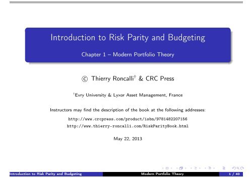
Introduction to Risk Parity and BudgetingChapter 1 – Modern Portfolio Theoryc○ Thierry Roncalli † & CRC Press† Evry University & Lyxor Asset Management, FranceInstructors may find the description of the book at the following addresses:http://www.crcpress.com/product/isbn/9781482207156http://www.thierry-roncalli.com/RiskParityBook.htmlMay 22, 2013Introduction to Risk Parity and Budgeting Modern Portfolio Theory 1 / 40

Figure 1.1, Page 6Figure: Optimized Markowitz portfoliosIntroduction to Risk Parity and Budgeting Modern Portfolio Theory 2 / 40

Figure 1.2, Page 8Figure: The efficient frontier of MarkowitzIntroduction to Risk Parity and Budgeting Modern Portfolio Theory 3 / 40

Table 1.1, Page 7Table: Solving the φ-problemφ +∞ 5.00 2.00 1.00 0.50 0.20x ⋆ 1 72.74 68.48 62.09 51.44 30.15 −33.75x ⋆ 2 49.46 35.35 14.17 −21.13 −91.72 −303.49x ⋆ 3 −20.45 12.61 62.21 144.88 310.22 806.22x ⋆ 4 −1.75 −16.44 −38.48 −75.20 −148.65 −368.99µ (x ⋆ ) 4.86 5.57 6.62 8.38 11.90 22.46σ (x ⋆ ) 12.00 12.57 15.23 22.27 39.39 94.57Introduction to Risk Parity and Budgeting Modern Portfolio Theory 4 / 40

Tables 1.2 & 1.3, Page 8Table: Solving the unconstrained µ-problemµ ⋆ 5.00 6.00 7.00 8.00 9.00x ⋆ 1 71.92 65.87 59.81 53.76 47.71x ⋆ 2 46.73 26.67 6.62 −13.44 −33.50x ⋆ 3 −14.04 32.93 79.91 126.88 173.86x ⋆ 4 −4.60 −25.47 −46.34 −67.20 −88.07σ (x ⋆ ) 12.02 13.44 16.54 20.58 25.10φ 25.79 3.10 1.65 1.12 0.85Table: Solving the unconstrained σ-problemσ ⋆ 15.00 20.00 25.00 30.00 35.00x ⋆ 1 62.52 54.57 47.84 41.53 35.42x ⋆ 2 15.58 −10.75 −33.07 −54.00 −74.25x ⋆ 3 58.92 120.58 172.85 221.88 269.31x ⋆ 4 −37.01 −64.41 −87.62 −109.40 −130.48µ (x ⋆ ) 6.55 7.87 8.98 10.02 11.03φ 2.08 1.17 0.86 0.68 0.57Introduction to Risk Parity and Budgeting Modern Portfolio Theory 5 / 40

Figure 1.3, Page 10Figure: The efficient frontier with some weight constraintsIntroduction to Risk Parity and Budgeting Modern Portfolio Theory 6 / 40

Table 1.4, Page 10Table: Solving the σ-problem with weight constraintsx i ∈ R x i ≥ 0 0 ≤ x i ≤ 40%σ ⋆ 15.00 20.00 15.00 20.00 15.00 20.00x ⋆ 1 62.52 54.57 45.59 24.88 40.00 6.13x ⋆ 2 15.58 −10.75 24.74 4.96 34.36 40.00x ⋆ 3 58.92 120.58 29.67 70.15 25.64 40.00x ⋆ 4 −37.01 −64.41 0.00 0.00 0.00 13.87µ (x ⋆ ) 6.55 7.87 6.14 7.15 6.11 6.74φ 2.08 1.17 1.61 0.91 1.97 0.28Introduction to Risk Parity and Budgeting Modern Portfolio Theory 7 / 40

Figure 1.4, Page 13Figure: The capital market lineIntroduction to Risk Parity and Budgeting Modern Portfolio Theory 8 / 40

Figure 1.5, Page 15Figure: The efficient frontier with a risk-free assetIntroduction to Risk Parity and Budgeting Modern Portfolio Theory 9 / 40

Tables 1.5 & 1.6, Pages 17 & 18Table: Computation of the betaPortfolio µ (y) β (y | x ⋆ ) π (y | x ⋆ )e 1 3.50 0.72 3.50e 2 4.50 0.92 4.50e 3 6.50 1.33 6.50e 4 4.50 0.92 4.50x ew 4.75 0.98 4.75Table: Computation of the beta with a constrained tangency portfolioPortfolio µ (y) β (y | x ⋆ ) π (y | x ⋆ )e 1 3.50 0.83 3.50e 2 4.50 1.06 4.50e 3 6.50 1.53 6.50e 4 4.50 1.54 6.53x ew 4.75 1.24 5.26Introduction to Risk Parity and Budgeting Modern Portfolio Theory 10 / 40

Figure 1.6, Page 20Figure: The efficient frontier with a benchmarkIntroduction to Risk Parity and Budgeting Modern Portfolio Theory 11 / 40

Figure 1.7, Page 22Figure: The tangency portfolio with respect to a benchmarkIntroduction to Risk Parity and Budgeting Modern Portfolio Theory 12 / 40

Table 1.7, Page 26Table: Black-Litterman portfolios#0 #1 #2 #3 #4 #5x ⋆ 1 40.00 33.41 51.16 36.41 38.25 39.77x ⋆ 2 30.00 51.56 39.91 42.97 42.72 32.60x ⋆ 3 20.00 5.46 0.00 10.85 9.14 17.65x ⋆ 4 10.00 9.58 8.93 9.77 9.89 9.98σ (x ⋆ | x 0 ) 0.00 3.65 3.67 2.19 2.18 0.45Introduction to Risk Parity and Budgeting Modern Portfolio Theory 13 / 40

Figure 1.8, Page 30Figure: Trading hours of asynchronous markets (UTC time)✬✩t m−1t m✉1:00❄✻7:001:00❄✻7:00Topix✲✉14:30❄✻21:0014:30❄✻21:00S&P 500✲✉8:00❄✻16:308:00❄✻16:30Eurostoxx✲✫✪Introduction to Risk Parity and Budgeting Modern Portfolio Theory 15 / 40

Figure 1.9, Page 31Figure: Density of the estimator ˆρ with asynchronous returnsIntroduction to Risk Parity and Budgeting Modern Portfolio Theory 16 / 40

Figure 1.10, Page 33Figure: Hayashi-Yoshida estimatorIntroduction to Risk Parity and Budgeting Modern Portfolio Theory 17 / 40

Figure 1.11, Page 35Figure: Cumulative weight W m of the IGARCH modelIntroduction to Risk Parity and Budgeting Modern Portfolio Theory 18 / 40

Figure 1.12, Page 36Figure: Estimation of the S&P 500 volatilityIntroduction to Risk Parity and Budgeting Modern Portfolio Theory 19 / 40

Figure 1.13, Page 38Figure: Density of the uniform correlation estimatorIntroduction to Risk Parity and Budgeting Modern Portfolio Theory 20 / 40

Result (1.19), Page 39Ĉ =⎛⎜⎝1.000.77 1.000.77 0.77 1.000.77 0.77 0.77 1.000.50 0.50 0.50 0.50 1.000.50 0.50 0.50 0.50 0.59 1.000.50 0.50 0.50 0.50 0.59 0.59 1.000.50 0.50 0.50 0.50 0.59 0.59 0.59 1.00⎞⎟⎠Introduction to Risk Parity and Budgeting Modern Portfolio Theory 21 / 40

Result (1.21), Page 39Ĉ =⎛⎜⎝1.000.88 1.000.88 0.94 1.000.63 0.67 0.66 1.000.73 0.78 0.78 0.63 1.000.58 0.62 0.60 0.54 0.59 1.000.56 0.59 0.58 0.56 0.60 0.54 1.000.64 0.68 0.66 0.65 0.69 0.62 0.67 1.00⎞⎟⎠Introduction to Risk Parity and Budgeting Modern Portfolio Theory 22 / 40

Table 1.8, Page 45Table: Sensitivity of the MVO portfolio to input parametersρ 70% 90% 90%σ 2 18% 18%µ 1 9%x 1 38.3 38.3 44.6 13.7 −8.0 60.6x 2 20.2 25.9 8.9 56.1 74.1 −5.4x 3 41.5 35.8 46.5 30.2 34.0 44.8Introduction to Risk Parity and Budgeting Modern Portfolio Theory 23 / 40

Figure 1.16, Page 46Figure: Uncertainty of the efficient frontierIntroduction to Risk Parity and Budgeting Modern Portfolio Theory 24 / 40

Figure 1.17, Page 48Figure: Resampled efficient frontierIntroduction to Risk Parity and Budgeting Modern Portfolio Theory 25 / 40

Result (1.23), Page 49Ĉ =⎛⎜⎝1.000.73 1.000.72 0.76 1.000.61 0.64 0.64 1.000.72 0.76 0.75 0.64 1.000.71 0.75 0.74 0.63 0.74 1.000.63 0.66 0.65 0.56 0.66 0.65 1.000.68 0.72 0.71 0.60 0.71 0.70 0.62 1.00⎞⎟⎠Introduction to Risk Parity and Budgeting Modern Portfolio Theory 26 / 40

Result (1.24), Page 51Ĉ =⎛⎜⎝1.000.77 1.000.77 0.80 1.000.65 0.67 0.65 1.000.72 0.71 0.72 0.63 1.000.61 0.64 0.63 0.58 0.65 1.000.60 0.64 0.62 0.60 0.63 0.62 1.000.65 0.67 0.67 0.67 0.67 0.63 0.66 1.00⎞⎟⎠Introduction to Risk Parity and Budgeting Modern Portfolio Theory 27 / 40

Table 1.9, Page 53Table: Solutions of penalized mean-variance optimizationMVO Ridge Lasso(NC) (C) (S) (D) (S) (D)x ⋆ 1 112.29 62.09 38.88 51.62 24.41 25.00x ⋆ 2 48.30 14.17 28.06 36.85 11.36 25.00x ⋆ 3 48.10 62.21 27.34 29.34 27.78 25.00x ⋆ 4 −39.69 −38.48 −1.57 −0.47 0.00 20.42Introduction to Risk Parity and Budgeting Modern Portfolio Theory 28 / 40

Figure 1.18, Page 54Figure: Weights of penalized MVO portfolios (in %)Introduction to Risk Parity and Budgeting Modern Portfolio Theory 29 / 40

Tables 1.10 & 1.11, Page 55Table: Principal component analysis of the covariance matrix ΣAsset / Factor 1 2 31 65.35% −72.29% −22.43%2 69.38% 69.06% −20.43%3 30.26% −2.21% 95.29%Eigenvalue 8.31% 0.84% 0.26%% cumulated 88.29% 97.20% 100.00%Table: Principal component analysis of the information matrix IAsset / Factor 1 2 31 −22.43% −72.29% 65.35%2 −20.43% 69.06% 69.38%3 95.29% −2.21% 30.26%Eigenvalue 379.97 119.18 12.04% cumulated 74.33% 97.65% 100.00%Introduction to Risk Parity and Budgeting Modern Portfolio Theory 30 / 40

Figure 1.19, Page 56Figure: PCA applied to the stocks of the FTSE index (June 2012)Introduction to Risk Parity and Budgeting Modern Portfolio Theory 31 / 40

Table 1.12, Page 57Table: Effect of deleting a PCA factorx ⋆ MV λ 1 = 0 λ 2 = 0 λ 3 = 0 λ 4 = 0 λ 5 = 0 λ 6 = 0x ⋆ 1 15.29 15.77 20.79 27.98 0.00 13.40 0.00x ⋆ 2 10.98 16.92 1.46 12.31 0.00 8.86 0.00x ⋆ 3 34.40 12.68 35.76 28.24 52.73 53.38 2.58x ⋆ 4 0.00 22.88 0.00 0.00 0.00 0.00 0.00x ⋆ 5 1.01 17.99 2.42 0.00 15.93 0.00 0.00x ⋆ 6 38.32 13.76 39.57 31.48 31.34 24.36 97.42Introduction to Risk Parity and Budgeting Modern Portfolio Theory 32 / 40

Table 1.13, Page 60Table: Limiting the turnover of MVO portfoliosτ + 5.00 10.00 25.00 50.00 75.00 x 0x ⋆ 1 35.00 36.40 42.34 45.59 30.00x ⋆ 2 45.00 42.50 30.00 24.74 45.00x ⋆ 3 15.00 21.10 27.66 29.67 15.00x ⋆ 4 5.00 0.00 0.00 0.00 10.00µ (x ⋆ ) 5.95 6.06 6.13 6.14 6.00σ (x ⋆ ) 15.00 15.00 15.00 15.00 15.69Introduction to Risk Parity and Budgeting Modern Portfolio Theory 33 / 40

Page 62Number of solved QP problemsn b n x Heuristic Backward Forward5010 40 1220 45540 10 455 122050050 450 123975 23775450 50 23775 1239751500100 1400 1120700 1450501000 500 625250 1000500Introduction to Risk Parity and Budgeting Modern Portfolio Theory 34 / 40

Table 1.14, Page 63Table: Sampling the SX5E index with the heuristic algorithmk Stock b i σ ( x (k) | b )1 Nokia 0.45 0.182 Carrefour 0.60 0.233 Repsol 0.71 0.284 Unibail-Rodamco 0.99 0.305 Muenchener Rueckver 1.34 0.326 RWE 1.18 0.367 Koninklijke Philips 1.07 0.418 Generali 1.06 0.459 CRH 0.82 0.5110 Volkswagen 1.34 0.5542 LVMH 2.39 3.6743 Telefonica 3.08 3.8144 Bayer 3.51 4.3345 Vinci 1.46 5.0246 BBVA 2.13 6.5347 Sanofi 5.38 7.2648 Allianz 2.67 10.7649 Total 5.89 12.8350 Siemens 4.36 30.33Introduction to Risk Parity and Budgeting Modern Portfolio Theory 35 / 40

Table 1.15, Page 63Table: Sampling the SX5E index with the backward elimination algorithmk Stock b i σ ( x (k) | b )1 Iberdrola 1.05 0.112 France Telecom 1.48 0.183 Carrefour 0.60 0.224 Muenchener Rueckver 1.34 0.265 Repsol 0.71 0.306 BMW 1.37 0.347 Generali 1.06 0.378 RWE 1.18 0.419 Koninklijke Philips 1.07 0.4410 Air Liquide 2.10 0.4842 GDF Suez 1.92 3.4943 Bayer 3.51 3.8844 BNP Paribas 2.26 4.4245 Total 5.89 4.9946 LVMH 2.39 5.7447 Allianz 2.67 7.1548 Sanofi 5.38 8.9049 BBVA 2.13 12.8350 Siemens 4.36 30.33Introduction to Risk Parity and Budgeting Modern Portfolio Theory 36 / 40

Table 1.16, Page 64Table: Sampling the SX5E index with the forward selection algorithmk Stock b i σ ( x (k) | b )1 Siemens 4.36 12.832 Banco Santander 3.65 8.863 Bayer 3.51 6.924 Eni 3.32 5.985 Allianz 2.67 5.116 LVMH 2.39 4.557 France Telecom 1.48 3.938 Carrefour 0.60 3.629 BMW 1.37 3.3541 Société Générale 1.07 0.5042 CRH 0.82 0.4543 Air Liquide 2.10 0.4144 RWE 1.18 0.3745 Nokia 0.45 0.3346 Unibail-Rodamco 0.99 0.2847 Repsol 0.71 0.2448 Essilor 1.17 0.1849 Muenchener Rueckver 1.34 0.1150 Iberdrola 1.05 0.00Introduction to Risk Parity and Budgeting Modern Portfolio Theory 37 / 40

Figure 1.20, Page 65Figure: Sampling the SX5E and SPX indicesIntroduction to Risk Parity and Budgeting Modern Portfolio Theory 38 / 40

Tables 1.17 & 1.18, Pages 68 & 69Table: Minimum variance portfolio when x i ≥ 10%˜x i λ −iλ +i˜σ i56.195 0.000 0.000 15.00 100.00˜ρ i,j23.805 0.000 0.000 20.00 10.00 100.0010.000 1.190 0.000 19.67 10.50 58.71 100.0010.000 1.625 0.000 23.98 17.38 16.16 67.52 100.00Table: Minimum variance portfolio when 10% ≤ x i ≤ 40%˜x i λ −iλ +i˜σ i40.000 0.000 0.915 20.20 100.00˜ρ i,j40.000 0.000 0.000 20.00 30.08 100.0010.000 0.915 0.000 21.02 35.32 61.48 100.0010.000 1.050 0.000 26.27 39.86 25.70 73.06 100.00Introduction to Risk Parity and Budgeting Modern Portfolio Theory 39 / 40

Tables 1.19 & 1.20, Pages 69 & 70Table: Mean-variance portfolio when 10% ≤ x i ≤ 40% and µ ⋆ = 6%˜x i λ −iλ +i˜σ i40.000 0.000 0.125 15.81 100.00˜ρ i,j30.000 0.000 0.000 20.00 13.44 100.0020.000 0.000 0.000 25.00 41.11 70.00 100.0010.000 1.460 0.000 24.66 23.47 19.06 73.65 100.00Table: MSR portfolio when 10% ≤ x i ≤ 40%˜x i λ −iλ +i˜σ i40.000 0.000 0.342 17.13 100.00˜ρ i,j39.377 0.000 0.000 20.00 18.75 100.0010.000 0.390 0.000 23.39 36.25 66.49 100.0010.623 0.000 0.000 30.00 50.44 40.00 79.96 100.00Introduction to Risk Parity and Budgeting Modern Portfolio Theory 40 / 40