Chapter 5 Student Lecture Notes 5-1 Distribusi ... - Blog Staff UI
Chapter 5 Student Lecture Notes 5-1 Distribusi ... - Blog Staff UI
Chapter 5 Student Lecture Notes 5-1 Distribusi ... - Blog Staff UI

You also want an ePaper? Increase the reach of your titles
YUMPU automatically turns print PDFs into web optimized ePapers that Google loves.
<strong>Chapter</strong> 5 <strong>Student</strong> <strong>Lecture</strong> <strong>Notes</strong> 5-1<br />
<strong>Distribusi</strong> Sampel<br />
<strong>Distribusi</strong> Sampel<br />
Sampling Distribution<br />
• Pengantar <strong>Distribusi</strong> Sampel<br />
• <strong>Distribusi</strong> mean Sampel dari Nilai Rata-rata<br />
• <strong>Distribusi</strong> mean Sampel dari Nilai Proporsi<br />
• <strong>Distribusi</strong> sampel adalah distribusi dari ratarata<br />
atau proporsi sampel yang diambil secara<br />
berulang-ulang (n kali) dari populasi.<br />
• Ada sebanyak n rata-rata atau n nilai proporsi<br />
• <strong>Distribusi</strong> dari rata-rata atau proporsi tersebut<br />
yang disebut sebagai distribusi sampel (sampling<br />
distribution)<br />
Chap 5-1<br />
Hal-2<br />
<strong>Distribusi</strong> Sampel<br />
• Sifat-sifat dari distribusi sampel tersebut dikenal<br />
dengan Central Limit Theorem f(X)<br />
1. Bentuk distribusi dari rata-rata sampel akan<br />
mendekati distrbusi normal meskipun distribusi<br />
populasi tidak normal.<br />
X<br />
2. Rata-rata dari rata-rata sampel sama dengan<br />
rata-rata populasi (µ)<br />
3. Standar deviasi dari rata-rata sampel sama<br />
dengan standar deviasi populasi (σ) dibagi<br />
dengan akar jumlah sampel. Dikenal dengan<br />
istilah Standard Error (SE) SE / n<br />
Hal-3<br />
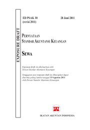
<strong>Distribusi</strong> Sampel<br />
• Asumsi suatu populasi<br />
• Besar Population N=4<br />
• Random variable, X,<br />
adalah umur<br />
• Nilai X: 18, 20,<br />
22, 24 dalam tahun<br />
A<br />
B C<br />
D<br />
Hal-4<br />
N<br />
<br />
X<br />
P(X)<br />
i<br />
i 1<br />
<br />
.3<br />
N<br />
.2<br />
18 20 22 24<br />
<br />
21<br />
4<br />
.1<br />
N<br />
2<br />
0<br />
X<br />
i<br />
<br />
i1<br />
<br />
2.236<br />
N<br />
<strong>Distribusi</strong> Sampel<br />
<strong>Distribusi</strong> Populasi<br />
(continued)<br />
A B C D X<br />
(18) (20) (22) (24)<br />
Uniform Distribution<br />
Hal-5<br />
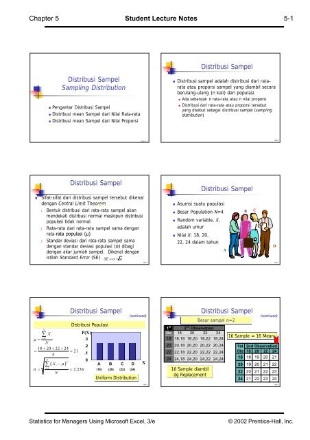
1 st 2 nd Observation<br />
Obs 18 20 22 24<br />
18 18,18 18,20 18,22 18,24<br />
20 20,18 20,20 20,22 20,24<br />
22 22,18 22,20 22,22 22,24<br />
24 24,18 24,20 24,22 24,24<br />
16 Sample diambil<br />
dg Replacement<br />
<strong>Distribusi</strong> Sampel<br />
Besar sampel n=2<br />
(continued)<br />
16 Sample = 16 Mean<br />
1st 2nd Observation<br />
Obs 18 20 22 24<br />
18 18 19 20 21<br />
20 19 20 21 22<br />
22 20 21 22 23<br />
24 21 22 23 24<br />
Hal-6<br />
Statistics for Managers Using Microsoft Excel, 3/e<br />
© 2002 Prentice-Hall, Inc.
<strong>Chapter</strong> 5 <strong>Student</strong> <strong>Lecture</strong> <strong>Notes</strong> 5-2<br />
Sampling Distribution of All Sample Means<br />
16 Sample Means<br />
1st 2nd Observation<br />
Obs 18 20 22 24<br />
18 18 19 20 21<br />
20 19 20 21 22<br />
22 20 21 22 23<br />
24 21 22 23 24<br />
<strong>Distribusi</strong> Sampel<br />
.3<br />
.2<br />
.1<br />
0<br />
P(X)<br />
Sample Means<br />
Distribution<br />
(continued)<br />
=Normal (3)<br />
18 19 20 21 22 23 24<br />
_<br />
X<br />
Hal-7<br />
<br />
N<br />
X<br />
18 19 19 <br />
24 21<br />
N 16<br />
N<br />
= mean populasi (1)<br />
2<br />
X <br />
i<br />
i1<br />
<br />
X<br />
<br />
X<br />
<br />
Sampling Distributions<br />
Summary Measures of Sampling Distribution<br />
<br />
<br />
i1<br />
i<br />
N<br />
X<br />
<br />
18 21 19 21 24 21<br />
<br />
2 2 2<br />
16<br />
1.58<br />
(continued)<br />
<br />
n SE..(2)<br />
Hal-8<br />
Perbandingan Populasi dan<br />
<strong>Distribusi</strong> Sampel<br />
<strong>Distribusi</strong> Sampling<br />
Population Sample Means Distribution<br />
N = 4<br />
n = 2<br />
21 2.236 21 1.58<br />
X<br />
X<br />
P(X)<br />
P(X)<br />
.3<br />
.3<br />
.2<br />
.2<br />
.1<br />
0<br />
A B C D<br />
(18) (20) (22) (24)<br />
X<br />
.1<br />
0<br />
18 19 20 21 22 23 24<br />
_<br />
X<br />
Hal-9<br />
Hal-10<br />
<strong>Distribusi</strong> Sampling<br />
x x x<br />
Z <br />
<strong>Distribusi</strong> probabilitas individu<br />
SD<br />
x x x <strong>Distribusi</strong> probabilitas rata-rata sampel<br />
Z <br />
/ n SD / n<br />
Contoh:<br />
Sampling Distribution<br />
2<br />
.4<br />
X<br />
25<br />
<br />
8 =2 n 25<br />
<br />
P 7.8 X 8.2 ?<br />
7.8<br />
8 X <br />
X<br />
8.2 8 <br />
P 7.8 X 8.2<br />
P <br />
2 / 25 <br />
X<br />
2 / 25 <br />
P .5 Z .5 .3830<br />
<br />
<br />
Standardized<br />
Normal Distribution<br />
<br />
Z<br />
1<br />
.1915<br />
Hal-11<br />
7.8<br />
8<br />
8.2 X 0.5<br />
0.5<br />
0<br />
Z<br />
X<br />
Z<br />
Hal-12<br />
Statistics for Managers Using Microsoft Excel, 3/e<br />
© 2002 Prentice-Hall, Inc.
<strong>Chapter</strong> 5 <strong>Student</strong> <strong>Lecture</strong> <strong>Notes</strong> 5-3<br />
<strong>Distribusi</strong> Probabilitas Individu<br />
<strong>Distribusi</strong> Sampel<br />
Contoh 1.<br />
Laporan tahunan RS ‘Sayang Ibu’ menyatakan bahwa ada sebanyak 500 kelahiran<br />
hidup selama setahun terakhir di RS tersebut. Rata-rata berat badan bayi adalah 3000<br />
gram dengan simpangan baku sebesar 500 gram. <strong>Distribusi</strong> berat badan bayi<br />
mengikuti distribusi normal. Bila Anda tertarik melihat data tersebut maka hitunglah<br />
probabilitas untuk mendapatkan berat bayi sebagai berikut:<br />
a. Bayi dengan berat badan bayi saat lahir lebih dari 3500 gram?<br />
b. Bayi dengan berat badan bayi saat lahir antara 2500 s/d 3500 gram?<br />
c. Bayi dengan berat badan bayi saat lahir 2000 s/d 2500 gram?<br />
d. Dinas Kesehatan di mana RS tersebut berada mengatakan bahwa ada sebesar<br />
20% kelahiran bayi BBLR (
<strong>Chapter</strong> 5 <strong>Student</strong> <strong>Lecture</strong> <strong>Notes</strong> 5-4<br />
Sampling Distribution<br />
p S<br />
<strong>Distribusi</strong> Sampel Proporsi<br />
pS <br />
p p<br />
S S<br />
p<br />
Z <br />
p 1<br />
p<br />
pS<br />
<br />
n<br />
<br />
Standardized<br />
Normal Distribution<br />
1<br />
Z<br />
Example:<br />
<br />
n 200 p .4 P p S<br />
.43 ?<br />
<br />
<br />
<br />
pS<br />
<br />
<br />
p .43 .4<br />
S<br />
P pS<br />
.43 P P Z<br />
.87 .8078<br />
<br />
p .41 .4<br />
S<br />
<br />
<br />
<br />
<br />
200 <br />
Sampling Distribution<br />
p S<br />
<br />
Standardized<br />
Normal Distribution<br />
1<br />
Z<br />
<br />
p S<br />
pS<br />
Z<br />
0<br />
Z<br />
Hal-19<br />
pS<br />
.43 p<br />
0 .87<br />
S<br />
Z<br />
Hal-20<br />
<strong>Distribusi</strong> Sampel Proporsi<br />
<strong>Distribusi</strong> Sampling<br />
Suatu survei di Kabupaten X pada tahun 2005 melaporkan bahwa prevalensi Anemia<br />
pada ibu hamil adalah sebesar 40%. Anda tertarik meneliti kejadian anemia ibu hamil<br />
di kabupaten X tersebut. Anda mencoba mengambil sampel secara acak sebanyak<br />
100 ibu hamil di Kabupaten X tersebut. Berapa probabilitas Anda akan mendapatkan<br />
bahwa ibu hamil dengan anemia sebagai berikut:<br />
a. Kurang dari 35%<br />
b. Lebih dari 45%<br />
c. Antara 35% s/d 45%<br />
Bila diambil sampel secara acak sebanyak 400 ibu hamil di Kabupaten X tersebut.<br />
Berapa probabilitas akan mendapatkan bahwa ibu hamil dengan anemia sebagai<br />
berikut:<br />
a. Kurang dari 35%<br />
b. Lebih dari 45%<br />
c. Antara 35% s/d 45%<br />
Hal-21<br />
1<br />
• Diketahui: P = 40% dan 1-P =<br />
60%<br />
• Sampel 100, Ditanya (c): P<br />
(antara 35% sampai 45%)?<br />
35 40% 45 x<br />
2<br />
0,35 0,40<br />
Z1 <br />
1,02<br />
0,40*(1 0,40)<br />
100<br />
-1.02 0<br />
1.02<br />
Z Lihat tabel Z arsir tengah<br />
3<br />
0,45 0,40<br />
Z1 <br />
1,02<br />
0,40*(1 0,40)<br />
100<br />
Z 1 p = 0.3461 (34,61%)<br />
Z 2 p = 0.3461 (34,61%)<br />
Total = 0.6922 (69,22%)<br />
Hal-22<br />
Sampling from Finite Sample<br />
• Modify standard error if sample size (n) is<br />
large relative to population size (N )<br />
• n .05 N or n / N .05<br />
• Use finite population correction factor (fpc)<br />
• Standard error with FPC<br />
•<br />
<br />
X<br />
•<br />
<br />
P S<br />
<br />
<br />
n<br />
<br />
<br />
N n<br />
N 1<br />
<br />
p 1<br />
p N n<br />
n N 1<br />
Hal-23<br />
Statistics for Managers Using Microsoft Excel, 3/e<br />
© 2002 Prentice-Hall, Inc.