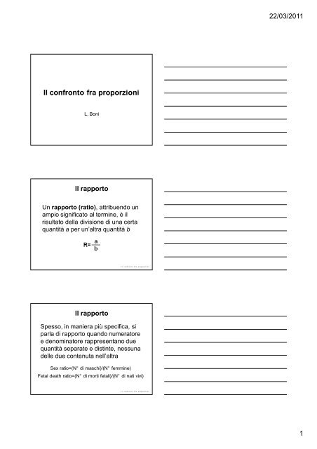
Il confronto fra proporzioni - Formazione e Sicurezza

Il confronto fra proporzioni
L. Boni
Il rapporto
Un rapporto (ratio), attribuendo un
ampio significato al termine, è il
risultato della divisione di una certa
quantità a per un’altra quantità b
Il rapporto
Il confronto fra proporzioni
Spesso, in maniera più specifica, si
parla di rapporto quando numeratore
e denominatore rappresentano due
quantità separate e distinte, nessuna
delle due contenuta nell’altra
Sex ratio=(N° di maschi)/(N° femmine)
Fetal death ratio=(N° di morti fetali)/(N° di nati vivi)
Il confronto fra proporzioni
22/03/2011
1

La proporzione
La proporzione è un particolare tipo
di rapporto in cui il numeratore è
compreso nel denominatore
La proporzione
Il confronto fra proporzioni
(N° di maschi) / [(N° di maschi) + (N° di femmine)]
Una proporzione ha sempre
numeratore e denominatore discreti
ed un valore compreso fra 0 e 1
Il confronto fra proporzioni
Come analizzare le proporzioni
FIGURA 5.1 GLANTZ
VARIABILE CASUALE BINARIA
P destro = P(X=0) = 150/200 = 0.75
P mancino = P(X=1) = 50/200 = 0.25
P destro = 1 - P mancino
Il confronto fra proporzioni
22/03/2011
2

Media di una variabile binaria
e generalizzando:
cioè la proporzione della popolazione con
la caratteristica studiata
Il confronto fra proporzioni
Deviazione standard di una variabile binaria
NOTA: Possiamo descrivere completamente
la struttura della popolazione con il singolo
parametro P
Il confronto fra proporzioni
Relazione fra media e deviazione
standard di una proporzione
FIGURA 5.3 GLANTZ
Il confronto fra proporzioni
22/03/2011
3

Stima di proporzioni
ottenute da campioni
Qual è la precisione con la quale la proporzione
di individui con un certa caratteristica di un
campione riflette la proporzione di individui con
la stessa caratteristica nella popolazione ?
FIGURA 5.4 GLANTZ
Stima di proporzioni
ottenute da campioni
FIGURA 5.5 GLANTZ
Il confronto fra proporzioni
Il confronto fra proporzioni
Errore standard della stima di
una proporzione
FIGURA 5.6 GLANTZ
Il confronto fra proporzioni
22/03/2011
4

Distribuzione binomiale
Distribuzione binomiale
Distribuzione binomiale
Il confronto fra proporzioni
Il confronto fra proporzioni
Il confronto fra proporzioni
22/03/2011
5

Distribuzione binomiale
dove
Assunti
Stiamo analizzando esperimenti di tipo
bernoulliano, nei quali:
Il confronto fra proporzioni
Ogni singolo esperimento ha solo due
possibili esiti mutuamente esclusivi
La probabilità P di un certo esito rimane
costante
Tutti gli esperimenti sono indipendenti
Assunti
Il confronto fra proporzioni
Utilizzando il concetto di popolazione,
possiamo riformulare gli assunti nel modo
seguente:
Ogni unità della popolazione appartiene
ad una sola delle due classi
La proporzione P di unità della
popolazione appartenenti ad una delle
due classi rimane costante
Ogni unità del campione è estratta
indipendentemente da tutte le altre unità
Il confronto fra proporzioni
22/03/2011
6

Confronto fra una proporzione
ed un valore atteso
RICORDA: Il teorema del limite
centrale afferma che la distribuzione di
p per campioni abbastanza numerosi è
approssimativamente normale con
media P e deviazione standard p
Il confronto fra proporzioni
Confronto fra una proporzione
ed un valore atteso
Se estraiamo ripetutamente un
campione di numerosità n da una
popolazione con parametro P, il 68%
dei campioni forniranno una stima di P
compresa nell’intervallo P 1 E.S. ed
il 95% nell’intervallo P 2 E.S.
Un esempio
Il confronto fra proporzioni
Il confronto fra proporzioni
22/03/2011
7

Un esempio
Questa approssimazione non vale per
valori di P vicini a 0 o a 1, o quando la
numerosità campionaria n è piccola.
Di regola è accettabile quando np e
n(1-p) sono entambi maggiori di 5.
Il confronto fra proporzioni
Confronto fra una proporzione
ed un valore atteso
P = parametro della popolazione
O/n = p = proporzione osservata
Ipotesi nulla (H0):
n è un campione casuale estratto da
una popolazione con parametro P
Il confronto fra proporzioni
Confronto fra una proporzione
ed un valore atteso
Test z:
misura in unità di D.S. (=E.S.) la
distanza fra la P della popolazione e
la p osservata
Il confronto fra proporzioni
22/03/2011
8

Confronto fra una proporzione
ed un valore atteso
Esempio: su 60 giocate alla roulette
mi aspetto 30 rossi (50%) e ne osservo
15
Il confronto fra proporzioni
Intervallo di confidenza di una
proporzione
Sappiamo che
segue approssimativamente la distribuzione
normale
Il confronto fra proporzioni
Intervallo di confidenza di una
proporzione
Ne deriva che
Nel nostro esempio:
0.25 - 1.96 x 0.064

Confronto fra due proporzioni
p 1 = O 1/n 1
p 2 = O 2/n 2
Ipotesi nulla (H0):
n 1 e n 2 sono due campioni casuali
estratti dalla stessa popolazione
p 1 = p 2 = P e p 1 - p 2 = 0
Il confronto fra proporzioni
Confronto fra due proporzioni
La migliore stima disponibile di P è la media
pesata tra p 1 e p 2, cioè:
Il confronto fra proporzioni
Confronto fra due proporzioni
Test z:
misura in unità di D.S. della differenza
(=E.S. d) la distanza tra la differenza
osservata (p 1-p 2) e quella attesa in base
all’ipotesi nulla (=0)
Il confronto fra proporzioni
22/03/2011
10

Un esempio
p(Trombo|Placebo) = 18/25 = 0.72
p(Trombo|Aspirina) = 6/19 = 0.32
verifichiamo:
25 x 0.72 = 18 e 25 x (1 - 0.72) = 7
19 x 0.32 = 6 e 19 x (1 - 0.32) = 13
Poiché tutti i valori sono più grandi di 5
possiamo applicare il metodo sviluppato
Un esempio
Il confronto fra proporzioni
Il confronto fra proporzioni
Intervallo di confidenza di una
differenza fra proporzioni
Sappiamo che:
segue approssimativamente la distribuzione
normale, da cui ne deriva che:
Il confronto fra proporzioni
22/03/2011
11

Intervallo di confidenza di una
differenza fra proporzioni
Nel nostro esempio:
0.40 - 1.96 x 0.15

Il test statistico chi quadrato
Il test statistico deve indicare la misura
con cui le frequenze osservate in ogni
cella della tabella differiscono dalle
frequenze che ci aspetteremmo, se non
ci fosse associazione fra i trattamenti e
gli esiti
Il confronto fra proporzioni
Il test statistico chi quadrato
Il test statistico deve inoltre tenere conto del
fatto che, nel caso in cui ci aspettiamo
parecchie osservazioni in una cella, la
differenza di una unità fra le frequenze attesa
ed osservata è meno importante che nel caso
in cui ci aspettiamo solo poche osservazioni
Distribuzione chi quadrato
Nel nostro esempio:
FIGURA 5.7 GLANTZ
Il confronto fra proporzioni
Il confronto fra proporzioni
22/03/2011
13

Distribuzione chi quadrato
L’utilizzo della distribuzione 2 presuppone
che, affinché la distribuzione teorica sia
un’approssimazione sufficientemente buona
di quella vera, il numero atteso di individui in
ogni cella sia uguale o maggiore di 5
E’ possibile dimostrare che 2 = z 2 quando ci
sono solo due campioni e due esiti possibili
Il confronto fra proporzioni
22/03/2011
14