A Short History of Assemblers and Loaders - David Salomon

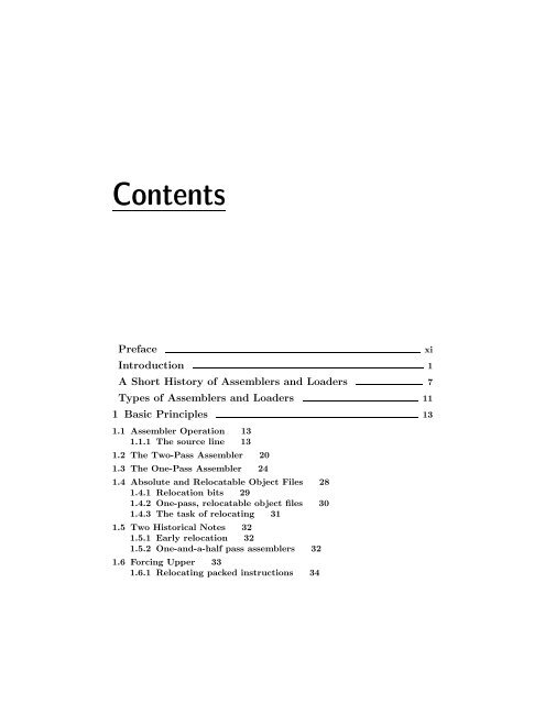
Contents
Preface xi
Introduction 1
A Short History of Assemblers and Loaders 7
Types of Assemblers and Loaders 11
1 Basic Principles 13
1.1 Assembler Operation 13
1.1.1 The source line 13
1.2 The Two-Pass Assembler 20
1.3 The One-Pass Assembler 24
1.4 Absolute and Relocatable Object Files 28
1.4.1 Relocation bits 29
1.4.2 One-pass, relocatable object files 30
1.4.3 The task of relocating 31
1.5 Two Historical Notes 32
1.5.1 Early relocation 32
1.5.2 One-and-a-half pass assemblers 32
1.6 Forcing Upper 33
1.6.1 Relocating packed instructions 34

vi Contents
1.7 Absolute and Relocatable Address Expressions 35
1.7.1 Summary 36
1.8 Local Labels 36
1.8.1 The LC as a local symbol 38
1.9 Multiple Location Counters 39
1.9.1 The USE directive 39
1.9.2 COMMON blocks 41
1.10 Literals 43
1.10.1 The literal table 43
1.10.2 Examples 44
1.11 Attributes of Symbols 45
1.12 Assembly-Time Errors 46
1.13 Review Questions and Projects 49
1.13.1 Project 1–1 50
1.13.2 Project 1–2 52
1.13.3 Project 1–3 53
1.13.4 Project 1–4 54
2 The Symbol Table 59
2.1 A Linear Array 60
2.2 A Sorted Array 60
2.3 Buckets with Linked Lists 61
2.4 A Binary Search Tree 62
2.5 A Hash Table 63
2.5.1 Closed hashing 63
2.5.2 Open hashing 65
2.6 Review Questions and Projects 66
2.6.1 Project 2–1 66
2.6.2 Project 2–2 66
2.6.3 Project 2–3 67
3 Directives 69
3.1 Introduction 69
3.2 Program Identification Directives 73
3.3 Source Program Control Directives 74
3.4 Machine Identification Directives 76
3.5 Loader Control Directives 77
3.6 Mode Control Directives 77
3.7 Block Control & LC Directives 79
3.8 Segment Control Directives 85
3.9 Symbol Definition Directives 86
3.10 Base Register Definition Directives 89

Contents vii
3.11 Subprogram Linkage Directives 90
3.12 Data Generation Directives 93
3.13 Macro Directives 99
3.14 Conditional Assembly Directives 99
3.15 Micro Directives 99
3.15.1 micro substitution 100
3.16 Error Control Directives 100
3.17 Listing Control Directives 101
3.18 Remote Assembly Directives 103
3.19 Code Duplication Directives 104
3.20 Operation Definition Directives 105
3.21 OpCode Table Management Directives 106
3.22 Summary 107
3.23 Review Questions and Projects 108
3.23.1 Project 3–1 108
3.23.2 Project 3–2 108
4 Macros 109
4.1 Introduction 109
4.1.1 The Syntax of macro definition and expansion 112
4.2 Macro Parameters 114
4.2.1 Properties of macro parameters 116
4.3 Operation of Pass 0 121
4.4 MDT Organization 122
4.4.1 The REMOVE directive 123
4.4.2 Order of search of the MDT 123
4.5 Other Features of Macros 124
4.5.1 Associating macro parameters with their arguments. 124
4.5.2 Delimiting macro parameters 125
4.5.3 Numeric values of arguments 125
4.5.4 Attributes of macro arguments 125
4.5.5 Directives related to arguments 126
4.5.6 Default arguments 127
4.5.7 Automatic label generation 127
4.5.8 The IRP directive 128
4.5.9 The PRINT directive 129
4.5.10 Comment lines in macros 129
4.6 Nested Macros 130
4.6.1 Nested macro expansion 130
4.7 Recursive Macros 133
4.8 Conditional Assembly 134
4.8.1 Global SET symbols 139

viii Contents
4.8.2 Array SET symbols 140
4.9 Nested Macro Definition 141
4.9.1 The traditional method 144
4.9.2 Revesz’s method 146
4.9.3 A note 154
4.10 Summary of Pass 0 154
4.11 Review Questions and Projects 156
4.11.1 Project 4–1 157
4.11.2 Project 4–2 157
5 The Listing File 159
5.1 A 6800 Example 160
5.2 A VAX Example 164
5.3 A MASM Example 169
5.4 An MPW Example 172
5.5 Review Questions and Projects 175
5.5.1 Project 5–1 175
6 Special Assembler Types 177
6.1 High-Level Assemblers 177
6.1.1 NEAT/3 178
6.1.2 PL360 181
6.1.3 PL516 183
6.1.4 BABBAGE 184
6.2 Summary 186
6.3 Meta Assemblers 186
6.4 Disassemblers 189
6.5 Cross Assemblers 193
6.6 Review Questions and Projects 194
6.6.1 Project 6–1 194
7 Loaders 195
7.1 Assemble-Go Loaders 196
7.2 Absolute Loaders 198
7.3 Linking Loaders 199
7.4 The Modify Loader Directive 209
7.5 Linkage Editors 211
7.6 Dymanic Linking 212
7.7 Loader Control 213
7.8 Library Routines 214
7.9 Overlays 215
7.10 Multiple Location Counters 219

Contents ix
7.11 Bootstrap Loaders 220
7.12 An N+1 address Assembler-Loader 221
7.13 Review Questions and Projects 224
7.13.1 Project 7–1 225
8 A Survey of Some Modern Assemblers 229
8.1 The Microsoft Macro Assembler (MASM) 230
8.1.1 The 80x86 & 80x88 microprocessors 230
8.1.2 MASM options 231
8.1.3 MASM listing 233
8.1.4 MASM source line format 233
8.1.5 MASM directives 233
8.1.6 MASM expressions 234
8.1.7 MASM macros 235
8.2 The Borland Turbo Assembler (TASM) 235
8.2.1 Special TASM features 236
8.2.2 TASM local labels 237
8.2.3 Automatic jump-sizing 237
8.2.4 Forward references to code and data 238
8.2.5 Conclusions: 239
8.2.6 TASM macros 239
8.2.7 The Ideal mode 239
8.2.8 TASM directives 240
8.3 The VAX Macro Assembler 240
8.3.1 Special Macro features 240
8.3.2 Data types 241
8.3.3 Local labels 242
8.3.4 Macro directives 242
8.3.5 Macros 243
8.3.6 Addressing modes 243
8.4 The Macintosh MPW Assembler 243
8.4.1 Modules 245
8.4.2 Listing file 245
8.4.3 Segments 246
8.4.4 Expressions & literals 246
8.4.5 Directives 246
References 249
A Addressing Modes 254
A.1 Introduction 254
A.2 Examples of Modes 256
A.2.1 The Direct mode 256
A.2.2 The Relative mode 257
A.2.3 The Immediate mode 257
A.2.4 The Index mode 258

x Contents
A.2.5 The Indirect mode 259
A.2.6 Multilevel or cascaded indirect 260
A.2.7 Other addressing modes 260
A.2.8 Zero Page mode 260
A.2.9 Current Page Direct mode 261
A.2.10 Implicit or Implied mode 261
A.2.11 Accumulator mode 261
A.2.12 Stack mode 261
A.2.13 Stack Relative mode 261
A.2.14 Register mode 262
A.2.15 Register Indirect mode 262
A.2.16 Auto Increment/Decrement mode 262
A.3 Base Registers 262
A.4 General Remarks 265
A.5 Review Questions 267
B Hexadecimal Numbers 268
B.1 Review Questions 270
C Answers to Exercises 271
Index 281

Preface
My computing experience dates back to the early 1960s, when higher-level languages
were fairly new.It is therefore no wonder that my introduction to computers
and computing came through assembler language; specifically, the IBM 7040 assembler
language.After programming in assembler exclusively (and enthusiastically)
for more than a year, I finally studied Fortran.However, my love affair with assemblers
has continued, and I very quickly discovered the lack of literature in this
field.In strict contrast to compilers, for which a wide range of literature exists,
very little has ever been written on assemblers and loaders.References [1,2,3,64]
are the best ones known to me, that describe and discuss the principles of operation
of assemblers and loaders.Assembler language textbooks are—of course—very
common, but they only talk about what assemblers do, not about how they do it.
One reason for this situation is that, for many years—from the mid 1950s to
the mid 1970s—assemblers were in decline.The development of Fortran and other
higher-level languages in the early 1950s overshadowed assemblers.The growth of
higher-level languages was taken by many a programmer to signal the demise of
assemblers, with the result that the use of assemblers dwindled.The advent of the
microprocessor, around 1975, caused a significant change, however.
Initially, there were no compilers available, so programmers had to use assemblers,
even primitive ones.This situation did not last long, of course, and today, in
the early 1990s, there are many compilers available for microcomputers, but assemblers
have not been neglected.Virtually all software development systems available

xii Preface
for modern computers include an assembler.The assemblers described in Ch.8 are
typical examples.
References [5–7] list three Z-80 assemblers running under CP/M.In spite of
being obsolete, they are good examples of modern assemblers.They are all state
of the art, relocatable assemblers that support macros and conditional assembly.
References [5,6] also include linking loaders.These assemblers reflect the interest
in the Z-80 and CP/M in the early 80s.Current processors, such as the 80x86 and
the 680x0 families, continue the tradition.Modern, sophisticated assemblers are
available for these processors, and are used extensively by programmers who need
optimized code in certain procedures.
The situation with loaders is different.Loaders have always been used.They
are used with as well as with assemblers, but their use is normally transparent to
the programmer.The average programmer hardly notices the existence of loaders,
which may explain the lack of literature in this area.
This book differs from the typical assembler text in that it is not a programming
manual, and it is not concerned with any specific assembler language.Instead
it concentrates on the design and implementation of assemblers and loaders.It
assumes that the reader has some knowledge of computers and programming, and it
aims to explain how assemblers and loaders work.Most of the discussion is general,
and most of the examples are in a hypothetical, simple, assembler language.Certain
examples are in the assembler languages of actual machines, and those are always
specified.Some good references for specific assembler languages are [5, 6, 7, 13, 26,
27, 30, 31, 32, 35, 37, 39, 101].
This work has its origins at a point, a few years ago, when my students started
complaining about a lack of literature in this field.Since I include assemblers and
loaders in classes that I teach every semester, I responded by developing class notes.
The notes were an immediate success, and have grown each semester, until I had
enough material for an expository paper on the subject.Since I was too busy to
polish the paper and submit it, I pretty soon found myself in a situation where the
work was too large for a paper.So here it is at last, in the form of a book.
This is mostly a professional book, intended for computer professionals in general,
and especially for systems programmers.However, it can be used as a supplementary
text in a systems programming or computer organization class at any
level.
Chapter 1 introduces the one-pass and two-pass assemblers, discusses other
important concepts—such as absolute- and relocatable object files—and describes
assembler features such as local labels and multiple location counters.
Data structures for implementing the symbol table are discussed in chapter 2.
Chapter 3 presents many directives and dicusses their formats, meaning, and
implementation.These directives are supported by many actual assemblers and,
while not complete, this collection of directives is quite extensive.
The two important topics of macros and conditional assembly are introduced
in chapter 4.The treatment of macros is as complete as practically possible.I have

Preface xiii
tried to include every possible feature of macros and the way it is implemented,
so this chapter can serve as a guide to practical macro implementation.At the
same time, I have tried not to concentrate on the macro features and syntax of any
specific assembler.
Features of the listing file are outlined, with examples, in chapter 5, while
chapter 6 is a general description of the properties of disassemblers, and of three
special types of assemblers.Those topics, especially meta-assemblers and high-level
assemblers, are of special interest to the advanced reader.They are not new, but
even experienced programmers are not always familiar with them.
Chapter 7 covers loaders.There is a very detailed example of the basic operation
of a one pass linking loader, followed by features and concepts such as dynamic
loading, bootstrap loader, overlays, and others.
Finally, chapter 8 contains a survey of four modern, state of the art, assemblers.
Their main characteristics are described, as well as features that distinguish them
from their older counterparts.
To make it possible to use the book as a textbook, each chapter is sprinkled
with exercises, all solved in appendix C.At the end of each chapter there are review
problems and projects.The review questions vary from very easy questions to tasks
that require the student to find some topic in textbooks and study it.The projects
are programming assignments, arranged from simple to more complex, that propose
various assemblers and loaders to be implemented.They should be done in the order
specified, since most of them are extensions of their predecessors.Some instructors
would find appendix A, on addressing modes, useful.
References are indicated by square brackets.Thus [14] (or Ref.[14]) refers to
Grishman’s book listed in the reference section.
This is the attention symbol.It is placed in front of paragraphs that require
special attention, that present fundamental concepts, or that are judged important
for other reasons.
Acknowledgement: I would like to acknowledge the help received from B.A.
Wichmann of the National Physical Laboratory in England.He sent me information
on the PL516 high-level assembler, the BABBAGE language, and the GE 4000
family of minicomputers.His was the only help I have received in collecting and
analyzing the material for this book.Johnny Tolliver, of Oak Ridge National Labs,
should also be mentioned.His version of the MakeIndex program proved invaluable
in preparing the extensive index of this book.
A human being; an ingenious assembly of portable plumbing
— Christopher Morley

Introduction
A work on assemblers should naturally start with a definition. However, computer
science is not as precise a field as mathematics, so most definitions are not
rigorous. The definition I like best is:
An assembler is a translator that translates source instructions
(in symbolic language) into target instructions
(in machine language), on a one to one basis.
This means that each source instruction is translated into exactly one target instruction.
This definition has the advantage of clearly describing the translation process
of an assembler. It is not a precise definition, however, because an assembler can
do (and usually does) much more than just translation. It offers a lot of help to
the programmer in many aspects of writing the program. The many types of help
offered by the assembler are grouped under the general term directives (or pseudoinstructions).
All the important directives are discussed in chapters 3 and 4.
Another good definition of assemblers is:
An assembler is a translator that translates a machineoriented
language into machine language.

2 Introduction
This definition distinguishes between assemblers and compilers. Compilers being
translators of problem-oriented languages or of machine-independent languages.
This definition, however, says nothing about the one-to-one nature of the translation,
and thus ignores a most important operating feature of an assembler.
One reason for studying assemblers is that the operation of an assembler reflects
the architecture of the computer. The assembler language depends heavily on
the internal organization of the computer. Architectural features such as memory
word size, number formats, internal character codes, index registers, and general
purpose registers, affect the way assembler instructions are written and the way the
assembler handles instructions and directives. This fact explains why there is an
interest in assemblers today and why a course on assembler language is still required
for many, perhaps even most, computer science degrees.
The first assemblers were simple assemble-go systems. All they could do was
to assemble code directly in memory and start execution. It was quickly realized,
however, that linking is an important feature, required even by simple programs.
The pioneers of programming have developed the concept of the routine library very
early, and they needed assemblers that could locate library routines, load them into
memory, and link them to the main program. It was this task of locating, loading,
and linking—of assembling a single working program from individual pieces—that
created the name assembler [4]. Today, assemblers are translators and they work
on one program at a time. The tasks of locating, loading, and linking (as well as
many other tasks) are performed by a loader.
A modern assembler has two inputs and two outputs. The first input is short,
typically a single line typed at a keyboard. It activates the assembler and specifies
the name of a source file (the file containing the source code to be assembled). It
may contain other information that the assembler should have before it starts. This
includes commands and specifications such as:
The names of the object file and listing file. Display (or do not display) the
listing on the screen while it is being generated. Display all error messages but do
not stop for any error. Save the listing file and do not print it (see below). This
program does not use macros. The symbol table is larger (or smaller) than usual
and needs a certain amount of memory.
All these terms are explained elsewhere. An example is the command line that
invokes Macro, the VAX assembler. The line:
MACRO /SHOW=MEB /LIST /DEBUG ABC
activates the assembler, tells it that the source program name is abc.mar (the .mar
extension is implied), that binary lines in macro expansions should be listed (shown),
that a listing file should be created, and that the debugger should be included in
the assembly.
Another typical example is the following command line that invokes the Microsoft
Macro assembler (MASM) for the 80x86 microprocessors:
MASM /d /Dopt=5 /MU /V

Introduction 3
It tells the assembler to create a pass 1 listing (/D), to create a variable opt and
set its value to 5, to convert all letters read from the source file to upper case (MU),
and to include certain information in the listing file (the V, or verbose, option).
The second input is the source file. It includes the symbolic instructions and
directives. The assembler translates each symbolic instruction into one machine
instruction. The directives, however, are not translated. The directives are our
way of asking the assembler for help. The assembler provides the help by executing
(rather than translating) the directives. A modern assembler can support as many
as a hundred directives. They range from ORG, which is very simple to execute,
to MACRO, which can be very complex. All the common directives are listed and
explained in chapters 3 and 4.
The first and most important output of the assembler is the object file. It
contains the assembled instructions (the machine language program) to be loaded
later into memory and executed. The object file is an important component of the
assembler-loader system. It makes it possible to assemble a program once, and later
load and run it many times. It also provides a natural place for the assembler to
leave information to the loader, instructing the loader in several aspects of loading
the program. This information is called loader directives and is covered in chapters
3 and 7. Note, however, that the object file is optional. The user may specify no
object file, in which case the assembler generates only a listing.
The second output of the assembler is the listing file. For each line in the source
file, a line is created in the listing file, containing:
The Location Counter (see chapter 1). The source line itself. The machine
instruction (if the source line is an instruction), or some other relevant information
(if the source line is a directive).
The listing file is generated by the assembler, sent to the printer, gets printed,
and is then discarded. The user, however, can specify either not to generate a listing
file or not to print it. There are also directives that control the listing. They can
be used to suppress parts of the listing, to print page headers, or to control the
printing of macro expansions.
The cross-reference information is normally a part of the listing file, although
the MASM assembler creates it in a separate file and uses a special utility to print
it. The cross-reference is a list of all symbols used in the program. For each symbol,
the point where it is defined and all the places where it is used, are listed.
Exercise .1 Why would anyone want to suppress the listing file or not to print it?
As mentioned above, the first assemblers were assemble-go type systems. They
did not generate any object file. Their main output was machine instructions loaded
directly into memory. Their secondary output was a listing. Such assemblers are
also in use today (for reasons explained in chapter 1) and are called one-pass assemblers.
In principle, a one pass assembler can produce an object file, but such a
file would be absolute and its use is limited.

4 Introduction
Most assemblers today are of the two-pass variety. They generate an object file
that is relocatable and can be linked and loaded by a loader.
A loader, as the name implies, is a program that loads programs into memory.
Modern loaders, however, do much more than that. Their main tasks (chapter
7) are loading, relocating, linking and starting the program. In a typical run,
a modern linking-loader can read several object files, load them one by one into
memory, relocating each as it is being loaded, link all the separate object files into
one executable module, and start execution at the right point. Using such a loader
has several advantages (see below), the most important being the ability to write
and assemble a program in several, separate, parts.
Writing a large program in several parts is advantageous, for reasons that will
be briefly mentioned but not fully discussed here. The individual parts can be
written by different programmers (or teams of programmers), each concentrating
on his own part. The different parts can be written in different languages. It is
common to write the main program in a higher-level language and the procedures in
assembler language. The individual parts are assembled (or compiled) separately,
and separate object files are produced. The assembler or compiler can only see one
part at a time and does not see the whole picture. It is only the loader that loads
the separate parts and combines them into a single program. Thus when a program
is assembled, the assembler does not know whether this is a complete program or
just a part of a larger program. It therefore assumes that the program will start at
address zero and assembles it based on that assumption. Before the loader loads the
program, it determines its true start address, based on the memory areas available
at that moment and on the previously loaded object files. The loader then loads the
program, making sure that all instructions fit properly in their memory locations.
This process involves adjusting memory addresses in the program, and is called
relocation.
Since the assembler works on one program at a time, it cannot link individual
programs. When it assembles a source file containing a main program, the assembler
knows nothing about the existence of any other source files containing, perhaps,
procedures called by the main program. As a result, the assembler may not be
able to properly assemble a procedure call instruction (to an external procedure) in
the main program. The object file of the main program will, in such a case, have
missing parts (holes or gaps) that the assembler cannot fill. The loader has access
to all the object files that make up the entire program. It can see the whole picture,
and one of its tasks is to fill up any missing parts in the object files. This task is
called linking.
The task of preparing a source program for execution includes translation (assembling
or compiling), loading, relocating, and linking. It is divided between the
assembler (or compiler) and the loader, and dual assembler-loader systems are very
common. The main exception to this arrangement is interpretation. Interpretive
languages such as BASIC or APL use the services of one program, the interpreter,
for their execution, and do not require an assembler or a loader. It should be clear
from the above discussion that the main reason for keeping the assembler and loader

Introduction 5
separate is the need to develop programs (especially large ones) in separate parts.
The detailed reasons for this will not be discussed here. We will, however, point out
the advantages of having a dual assembler-loader system. They are listed below, in
order of importance.
It makes it possible to write programs in separate parts that may also be in
different languages.
It keeps the assembler small. This is an important advantage. The size of the
assembler depends on the size of its internal tables (especially the symbol table and
the macro definition table). An assembler designed to assemble large programs is
large because of its large tables. Separate assembly makes it possible to assemble
very large programs with a small assembler.
When a change is made in the source code, only the modified program needs to
be reassembled. This property is a benefit if one assumes that assembly is slow and
loading is fast. Many times, however, loading is slower than assembling, and this
property is just a feature, not an advantage, of a dual assembler-loader system.
The loader automatically loads routines from a library. This is considered by
some an advantage of a dual assembler-loader system but, actually, it is not. It
could easily be done in a single assembler-loader program. In such a program, the
library would have to contain the source code of the routines, but this is typically
not larger than the object code.

6 Introduction
The words of the wise are as goads, and as nail fastened by masters of
assemblies
— Ecclesiastes 12:11

A Short History of
Assemblers and Loaders
One of the first stored program computers was the EDSAC (Electronic Delay
Storage Automatic Calculator) developed at Cambridge University in 1949 by
Maurice Wilkes and W. Renwick [4, 8 & 97]. From its very first days the EDSAC
had an assembler, called Initial Orders. It was implemented in a read-only memory
formed from a set of rotary telephone selectors, and it accepted symbolic instructions.
Each instruction consisted of a one letter mnemonic, a decimal address, and
a third field that was a letter. The third field caused one of 12 constants preset by
the programmer to be added to the address at assembly time.
It is interesting to note that Wilkes was also the first to propose the use of
labels (which he called floating addresses), the first to use an early form of macros
(which he called synthetic orders), and the first to develop a subroutine library [4].
Reference [65] is a very early description of the use of labels in an assembler The
IBM 650 computer was first delivered around 1953 and had an assembler very similar
to present day assemblers. SOAP (Symbolic Optimizer and Assembly Program) did
symbolic assembly in the conventional way, and was perhaps the first assembler to
do so. However, its main feature was the optimized calculation of the address of
the next instruction. The IBM 650 (a decimal computer, incidentally), was based
on a magnetic drum memory and the program was stored in that memory. Each

8 A Short History of Assemblers and Loaders
instruction had to be fetched from the drum and had to contain the address of
its successor. For maximum speed, an instruction had to be placed on the drum
in a location that would be under the read head as soon as its predecessor was
completed. SOAP calculated those addresses, based on the execution times of the
individual instructions. Chapter 7 has more details, and a programming project,
on this process.
One of the first commercially successful computers was the IBM 704. It had
features such as floating-point hardware and index registers. It was first delivered
in 1956 and its first assembler, the UASAP-1, was written in the same year by Roy
Nutt of United Aircraft Corp. (hence the name UASAP—United Aircraft Symbolic
Assembly Program). It was a simple binary assembler, did practically nothing
but one-to-one translation, and left the programmer in complete control over the
program. SHARE, the IBM users’ organization, adopted a later version of that
assembler [9] and distributed it to its members together with routines produced
and contributed by members. UASAP has pointed the way to early assembler
writers, and many of its design principles are used by assemblers to this day. The
UASAP was later modified to support macros [62].
In the same year another assembler, the IBM Autocoder was developed by R.
Goldfinger [10] for use on the IBM 702/705 computers. This assembler (actually
several different Autocoder assemblers) was apparently the first to use macros. The
Autocoder assemblers were used extensively and were eventually developed into
large systems with large macro libraries used by many installations.
Another pioneering early assembler was the UNISAP, [47] for the UNIVAC I
& II computers, developed in 1958 by M. E. Conway. It was a one-and-a-half pass
assembler, and was the first one to use local labels. Both concepts are covered in
chapter 1.
By the late fifties, IBM had released the 7000 series of computers. These came
with a macro assembler, SCAT, that had all the features of modern assemblers.
It had many directives (pseudo instructions in the IBM terminology), an extensive
macro facility, and it generated relocatable object files.
The SCAT assembler (Symbolic Coder And Translator) was originally written
for the IBM 709 [56] and was modified to work on the IBM 7090. The GAS (Generalized
Assembly System) assembler was another powerful 7090 assembler [58].
The idea of macros originated with several people. McIlroy [22] was probably
the first to propose the modern form of macros and the idea of conditional assembly.
He implemented these ideas in the GAS assembler mentioned above. Reference [60]
is a short early paper presenting some details of macro definition table handling.
One of the first full-feature loaders, the linking loader for the IBM 704–709–
7090 computers [59], is an example of an early loader supporting both relocation
and linking.
The earliest work discussing meta-assemblers seems to be Ferguson [24]. The
idea of high-level assemblers originated with Wirth [61] and had been extended,

Relocation
Bits
External
Relocatable
Routines
Relocatable
Assembler
and Loader
A Short History of Assemblers and Loaders 9
Machine Language
Assembler Language
Directives
Absolute Assembler
External
Routines
Absolute Assembler
with
Library Routines
Linking Loader Macros
Macro Assembler
Conditional Assembly
Full-Feature, Relocatable
Macro Assembler, with
Conditional Assembly
Phases in the historical development of assemblers and loaders.

10 A Short History of Assemblers and Loaders
a few years later, by an anonymous software designer at NCR, who proposed the
main ideas of the NEAT/3 language [85,86].
The diagram summarizes the main phases in the historical development of
assemblers and loaders.
I would like to present a brief historical background as a preface to the
language specification contained in this manual.
— John Warnock Postscript Language Reference Manual, 1985.

Types of
Assemblers and Loaders
A One-pass Assembler: One that performs all its functions by reading the source
file once.
A Two-Pass Assembler: One that reads the source file twice.
A Resident Assembler: One that is permanently loaded in memory. Typically
such an assembler resides in ROM, is very simple (supports only a few directives
and no macros), and is a one-pass assembler. The above assemblers are described
in chapter 1.
A Macro-Assembler: One that supports macros (chapter 4).
A Cross-Assembler: An assembler that runs on one computer and assembles programs
for another. Many cross-assemblers are written in a higher-level language to
make them portable. They run on a large machine and produce object code for a
small machine.
A Meta-Assembler: One that can handle many different instruction sets.
A Disassembler: This, in a sense, is the opposite of an assembler. It translates
machine code into a source program in assembler language.

12 Types of Assemblers and Loaders
A high-level assembler. This is a translator for a language combining the features
of a higher-level language with some features of assembler language. Such a language
can also be considered a machine dependent higher-level language. The above four
types are described in chapter 6.
A Micro-Assembler: Used to assemble microinstructions. It is not different in
principle from an assembler. Note that microinstructions have nothing to do with
programming microcomputers.
Combinations of those types are common. An assembler can be a Macro Cross-
Assembler or a Micro Resident one.
A Bootstrap Loader: It uses its first few instructions to either load the rest of
itself, or load another loader, into memory. It is typically stored in ROM.
An Absolute Loader: Can only load absolute object files, i.e., can only load a
program starting from a certain, fixed location in memory.
A Relocating Loader: Can load relocatable object files and thus can load the same
program starting at any location.
A Linking Loader: Can link programs that were assembled separately, and load
them as a single module.
A Linkage Editor: Links programs and does some relocation. Produces a load
module that can later be loaded by a simple relocating loader. All loader types are
discussed in chapter 7.

1. Basic Principles
The basic principles of assembler operation are simple, involving just one problem,
that of unresolved references. This is a simple problem that has two simple
solutions. The problem is important, however, since its two solutions introduce,
in a natural way, the two main types of assemblers namely, the one-pass and the
two-pass.
1.1 Assembler Operation
As mentioned in the introduction, the main input of the assembler is the source
file. Each record on the source file is a source line that specifes either an assembler
instruction or a directive.
1.1.1 The source line
A typical source line has four fields. A label (or a location), a mnemonic (or
operation), an operand, and a comment.
Example: LOOP ADD R1,ABC PRODUCING THE SUM
In this example, LOOP is a label, ADD is a mnemonic meaning to add, R1 stands
for register 1, and ABC is the label of another source line. R1 and ABC are two
operands that make up the operand field. The example above is, therefore, a doubleoperand
instruction. When a label is used as an operand, we call it a symbol. Thus,
in our case, ABC is a symbol.

14 Basic Principles Ch. 1
The comment is for the programmer’s use only. It is read by the assembler, it
is listed in the listing file, and is otherwise ignored.
The label field is only necessary if the instruction is referred to from some
other point in the program. It may be referred to by another instruction in the
same program, by another instruction in a different program (the two programs
should eventually be linked), or by itself.
The word mnemonic comes from the Greek µνɛµoνικoσ, meaning pertaining to
memory; it is a memory aid. The mnemonic is always necessary. It is the operation.
It tells the assembler what instruction needs to be assembled or what directive to
execute (but see the comment below about blank lines).
The operand depends on the mnemonic. Instructions can have zero, one, or
two operands (very few computers have also three operand instructions). Directives
also have operands. The operands supply information to the assembler about the
source line.
As a result, only the mnemonic is mandatory, but there are even exceptions
to this rule. One exception is blank lines. Many assemblers allow blank lines—in
which all fields, including the mnemonic, are missing—in the source file. They make
the listing more readable but are otherwise ignored.
Another exception is comment lines. A line that starts with a special symbol
(typically a semicolon, sometimes an asterisk and, in a few cases, a slash)is
considered a comment line and, of course, has no mnemonic. Many modern assemblers
(see, e.g., references [37], [99]–[102])support a COMMENT directive that has the
following form:
COMMENT delimiter text delimiter
Where the text between the delimiters is a comment. This way the programmer
can enter a long comment, spread over many lines, without having to start each
line with the special comment symbol. Example:
COMMENT =This is a long
comment that ...
.
.
... sufficient to describe what you want=
Old assemblers were developed on punched-card based computers. They required
the instructions to be punched on cards such that each field of the source
line was punched in a certain field on the card. The following is an example from
the IBMAP (Macro Assembler Program)assembler for the IBM 7040 [12]. A source
line in this assembler has to be punched on a card with the format:

Sec. 1.1 Assembler Operation 15
and also obey the following rules:
Columns Field
1-6 Label
7 Blank
8- Mnemonic
The operand must be separated from the mnemonic by at least one blank, and
must start on or before column 16.
The comment must be separated from the operand by at least one blank. If there
is no operand, the comment may not start before column 17.
The comment extends through column 80 but columns 73–80 are normally used
for sequencing and identification.
It is obviously very hard to enter such source lines from a keyboard. Modern
assemblers are thus more flexible and do not require any special format. If a label
exists, it must end with a ‘:’. Otherwise, the individual fields should be separated
by at least one space (or by a tab character), and subfields should be separated by
either a comma or parentheses. This rule makes it convenient to enter source lines
from a keyboard, but is ambiguous in the case of a source line that has a comment
but no operand.
Example: EI ;ENABLE ALL INTERRUPTS
The semicolon guarantees that the word ENABLE will not be considered an
operand by the assembler. This is why many assemblers require that comments
start with a semicolon.
Exercise 1.1 Why a semicolon and not some other character such as ‘$’ or ‘@’ ?
Many modern assemblers allow labels without an identifying ‘:’. They simply
have to work harder in order to identify labels.
The instruction sets of some computers are designed such that the mnemonic
specifies more than just the operation. It may also contain part of the operand.
The Signetics 2650 microprocessor, for example, has many mnemonics that include
one of the operands [13]. A ‘Store Relative’ instruction on the 2650 may be written
STRR,R0 SAV; the mnemonic field includes R0 (the register to be stored in location
SAV), which is an operand.
On other computers, the operation may partly be specified in the operand
field. The instruction IX7 X2+X5, on the CDC Cyber computers [14] means: “add
register X2 and register X5 as integers, and store the sum in register X7.” The
operation appears partly in the operation field (‘I’)and partly in the operand field
(‘+’), whereas X7 (an operand)appears in the mnemonic. This makes it harder
for the assembler to identify the operation and the operands and, as a result, such
instruction formats are not common.

16 Basic Principles Ch. 1
Exercise 1.2 What is the meaning of the Cyber instruction FX7 X2+X5?
To translate an instruction, the assembler uses the OpCode table, which is a
static data structure. The two important columns in the table are the mnemonic
and OpCode. Table 1–1 is an example of a simple OpCode table. It is part of the
IBM 360 OpCode table and it includes other information.
mnemonic OpCode type length
A 5A RX 4
AD 6A RX 4
ADR 2A RR 2
AER 3A RR 2
AE 1A RR 2
Table 1–1
The mnemonics are from one to four letters long (in many assemblers they
may include digits). The OpCodes are two hexadecimal digits (8 bits) long, and the
types (which are irrelevant for now)provide more information to the assembler.
The OpCode table should allow for a quick search. For each source line input,
the assembler has to search the OpCode table. If it finds the mnemonic, it uses the
OpCode to start assembling the instruction. It also uses the other information in
the OpCode table to complete the assembly. If it does not find the mnemonic in the
table, it assumes that the mnemonic is that of a directive and proceeds accordingly
(see chapter 3).
The OpCode table thus provides for an easy first step of assembling an instruction.
The next step is using the operand to complete the assembly. The OpCode
table should contain information about the number and types of operands for each
instruction. In table 1–1 above, the type column provides this information. Type
RR means a Register-Register instruction. This is an instruction with two operands,
both registers. The assembler expects two operands, both numbers between 0 and
15 (the IBM 360 has 16 general-purpose registers). Each register number is assembled
as a 4 bit field.
Exercise 1.3 Why does the IBM 360 have 16 general purpose registers and not a
round number such as 15 or 20?
Example: The instruction ‘AR 4,6’ means: add register 6 (the source)to register
4 (the destination operand). It is assembled as the 16-bit machine instruction
1A46, in which 1A is the OpCode and 46, the two operands.
Type RX stands for Register-indeX. In these instructions the operand consists
of a register followed by an address.
Example: ‘BAL 5,14’. This instruction calls a procedure at location 14, and
saves the return address in register 5 (BAL stands for Branch And Link). It is
assembled as the 32-bit machine instruction 4550000E in which 00E is a 12-bit

Sec. 1.1 Assembler Operation 17
address field (E is hexadecimal 14), 45 is the OpCode, 5 is register 5, and the two
zeros in the middle are irrelevant to our discussion. (A note to readers familiar
with the IBM 360—This example ignores base registers as they do not contribute
anything to our discussion of assemblers.)
Exercise 1.4 What are the two zeros in the middle of the instruction used for?
This example is not a typical one. Numeric addresses are rarely used in assembler
programming, since keeping track of their values is a tedious task better left to
the assembler. In practice, symbols are used instead of numeric addresses. Thus the
above example is likely to be written as ‘BAL 5,XYZ’, where XYZ is a symbol whose
value is an address. Symbol XYZ should be the label of some source line. Typically
the program will contain the two lines
XYZ A 4,ABC ;THE SUBROUTINE STARTS HERE
.
.
BAL 5,XYZ ;THE SUBROUTINE IS CALLED
Besides the basic task of assembling instructions, the assembler offers many
services to the user, the most important of which is handling symbols. This task
consists of two different parts, defining symbols, and using them. A symbol is
defined by writing it as a label. The symbol is used by writing it in the operand
field of a source line. A symbol can only be defined once but it can be used any
number of times. To understand how a value is assigned to a symbol, consider the
example above. The ‘add’ instruction A is assembled and is eventually loaded into
memory as part of the program. The value of symbol XYZ is the memory address of
that instruction. This means that the assembler has to keep track of the addresses
where instructions are loaded, since some of them will become values of symbols.
To do this, the assembler uses two tools, the location counter (LC), and the symbol
table.
The LC is a variable, maintained by the assembler, that contains the address
into which the current instruction will eventually be loaded. When the assembler
starts, it clears the LC, assuming that the first instruction will go into location 0.
After each instruction is assembled, the assembler increments the LC by the size
of the instruction (the size in words, not in bits). Thus the LC always contains
the current address. Note that the assembler does not load the instructions into
memory. It writes them on the object file, to be eventually loaded into memory by
the loader. The LC, therefore, does not point to the current instruction. It just
shows where the instruction will eventually be loaded. When the source line has
a label (a newly defined symbol), the label is assigned the current value of the LC
as its value. Both the label and its value (plus some other information)are then
placed in the symbol table.
The symbol table is an internal, dynamic table that is generated, maintained,
and used by the assembler. Each entry in the table contains the definition of a
symbol and has fields for the name, value, and type of the symbol. Some symbol

18 Basic Principles Ch. 1
tables contain other information about the symbols. The symbol table starts empty,
labels are entered into it as their definitions are found in the source, and the table
is also searched frequently to find the values and types of symbols whose names are
known. Chapter 2 discusses various ways to implement symbol tables.
In the above example, when the assembler encounters the line
XYZ A 5,ABC ;THE SUBROUTINE STARTS HERE
it performs two independent operations. It stores symbol XYZ and its value (the
current value of the LC)in the symbol table, and it assembles the instruction.
These two operations have nothing to do with each other. Handling the symbol
definition and assembling the instruction are done by two different parts of the
assembler. Many times they are performed in different phases of the assembly.
If the LC happens to have the value 260, then the entry
name value type
XYZ 0104 REL
will be added to the symbol table (104 is the hex value of decimal 260, and the type
REL will be explained later).
When the assembler encounters the line
BAL 5,XYZ
it assembles the instruction but, in order to assemble the operand, the assembler
needs to search the symbol table, find symbol XYZ, fetch its value and make it part
of the assembled instruction. The instruction is, therefore, assembled as 45500104.
Exercise 1.5 The address in our example, 104, is a relatively small number. Many
times, instructions have a 12-bit field for the address, allowing addresses up to
2 12 − 1 = 4095. What if the value of a certain symbol exceeds that number?
This is, in a very general way, what the assembler has to do in order to assemble
instructions and handle symbols. It is a simple process and it involves only one
problem which is illustrated by the following example.
BAL 5,XYZ ;CALL THE SUBROUTINE
.
.
XYZ A 4,ABC ;THE SUBROUTINE STARTS HERE
In this case the value of symbol XYZ is needed before label XYZ is defined. When the
assembler gets to the first line (the BAL instruction), it searches the symbol table
for XYZ and, of course, does not find it. This situation is called the future symbol
problem or the problem of unresolved references. The XYZ in our example is a future
symbol or an unresolved reference.

Sec. 1.1 Assembler Operation 19
Obviously, future symbols are not an error and their use should not be prohibited.
The programmer should be able to refer to source lines which either precede
or follow the current line. Thus the future symbol problem has to be solved. It
turns out to be a simple problem and there are two solutions, a one-pass assembler
and a two-pass assembler. They represent not just different solutions to the future
symbol problem but two different approaches to assembler design and operation.
The one-pass assembler, as the name implies, solves the future symbol problem
by reading the source file once. Its most important feature, however, is that it
does not generate a relocatable object file but rather loads the object code (the
machine language program)directly into memory. Similarly, the most important
feature of the two-pass assembler is that it generates a relocatable object file, that
is later loaded into memory by a loader. It also solves the future symbol problem
by performing two passes over the source file. It should be noted at this point that
a one-pass assembler can generate an object file. Such a file, however, would be
absolute, rather than relocatable, and its use is limited. Absolute and relocatable
object files are discussed later in this chapter. Figure 1–1 is a summary of the most
important components and operations of an assembler.
Source
file
Source line
buffer
Lexical scan
routine
Opcode
table
Pass
indicator
Main
Program
Location counter
Table search procedures
Directive
table
Symbol
table
Error
proc.
Object
code
assembly
area
Object
file
Figure 1–1. The Main Components andOperations of an Assembler.

20 Basic Principles Ch. 1
1.2 The Two-Pass Assembler
A two-pass assembler is easier to understand and will be discussed first. Such
an assembler performs two passes over the source file. In the first pass it reads the
entire source file, looking only for label definitions. All labels are collected, assigned
values, and placed in the symbol table in this pass. No instructions are assembled
and, at the end of the pass, the symbol table should contain all the labels defined in
the program. In the second pass, the instructions are again read and are assembled,
using the symbol table.
Exercise 1.6 What if a certain symbol is needed in pass 2, to assemble an instruction,
and is not found in the symbol table?
To assign values to labels in pass 1, the assembler has to maintain the LC. This
in turn means that the assembler has to determine the size of each instruction (in
words), even though the instructions themselves are not assembled.
In many cases it is easy to figure out the size of an instruction. On the IBM 360,
the mnemonic determines the size uniquely. An assembler for this machine keeps
the size of each instruction in the OpCode table together with the mnemonic and
the OpCode (see table 1–1). On the DEC PDP-11 the size is determined both
by the type of the instruction and by the addressing mode(s)that it uses. Most
instructions are one word (16-bits)long. However, if they use either the index or
index deferred modes, one more word is added to the instruction. If the instruction
has two operands (source and destination)both using those modes, its size will be
3 words. On most modern microprocessors, instructions are between 1 and 4 bytes
long and the size is determined by the OpCode and the specific operands used.
This means that, in many cases, the assembler has to work hard in the first
pass just to determine the size of an instruction. It has to look at the mnemonic
and, sometimes, at the operands and the modes, even though it does not assemble
the instruction in the first pass. All the information about the mnemonic and
the operand collected by the assembler in the first pass is extremely useful in the
second pass, when instructions are assembled. This is why many assemblers save
all the information collected during the first pass and transmit it to the second pass
through an intermediate file. Each record on the intermediate file contains a copy
of a source line plus all the information that has been collected about that line in
the first pass. At the end of the first pass the original source file is closed and is no
longer used. The intermediate file is reopened and is read by the second pass as its
input file.
A record in a typical intermediate file contains:
The record type. It can be an instruction, a directive, a comment, or an invalid
line.
The LC value for the line.
A pointer to a specific entry in the OpCode table or the directive table. The
second pass uses this pointer to locate the information necessary to assemble or
execute the line.

Sec. 1.2 The Two-Pass Assembler 21
A copy of the source line. Notice that a label, if any, is not use by pass 2 but
must be included in the intermediate file since it is needed in the final listing.
Fig. 1–2 is a flow chart summarizing the operations in the two passes.
There can be two problems with labels in the first pass; multiply-defined labels
and invalid labels. Before a label is inserted into the symbol table, the table has to
be searched for that label. If the label is already in the table, it is doubly (or even
multiply-)defined. The assembler should treat this label as an error and the best
way of doing this is by inserting a special code in the type field in the symbol table.
Thus a situation such as:
AB ADD 5,X
.
.
AB SUB 6,Y
.
.
JMP AB
will generate the entry:
in the symbol table.
name value type
AB — MTDF
Labels normally have a maximum size (typically 6 or 8 characters), must start
with a letter, and may only consist of letters, digits, and a few other characters.
Labels that do not conform to these rules are invalid labels and are normally considered
a fatal error. However, some assemblers will truncate a long label to the
maximum size and will issue just a warning, not an error, in such a case.
Exercise 1.7 What is the advantage of allowing characters other than letters and
digits in a label?
The only problem with symbols in the second pass is bad symbols. These are
either multiply-defined or undefined symbols. When a source line uses a symbol in
the operand field, the assembler looks it up in the symbol table. If the symbol is
found but has a type of MTDF, or if the symbol is not found in the symbol table (i.e.,
it has not been defined), the assembler responds as follows.
It flags the instruction in the listing file.
It assembles the instruction as far as possible, and writes it on the object file.
It flags the entire object file. The flag instructs the loader not to start execution
of the program. The object file is still generated and the loader will read and load
it, but not start it. Loading such a file may be useful if the user wants to see a
memory map (see discussion of memory maps in chapter 7).

22 Basic Principles Ch. 1
pass 1
read line
from source file
eof
?
no
label
defined
?
no
determine size
of instruction
LC:=LC+size
1
yes
write source line & other
info on intermediate file
yes
1
close source file
rewind intermediate
file
pass 2
store name & value
in symbol table
Figure 1–2. The Operations of the Two-Pass Assmbler (part 1).
The JMP AB instruction above is an example of a bad symbol in the operand
field. This instruction cannot be fully assembled, and thus constitutes our first
example of a fatal error detected and issued by the assembler.
The last important point regarding a two-pass assembler is the box, in the flow
chart above, that says write object instruction onto the object file. The point is that
when the two-pass assembler writes the machine instruction on the object file, it has
access to the source instruction. This does not seem to be an important point but,
in fact, it constitutes the main difference between the one-pass and the two-pass

Sec. 1.2 The Two-Pass Assembler 23
2
stop
yes
pass 2
read next line from
intermediate file
eof
?
2
no
assemble
instruction
write object instruction
onto object file
write source & object
lines onto listing file
Figure 1–2. The Operations of the Two-Pass Assmbler (part 2).
assemblers. This point is the reason why a one-pass assembler can only produce
an absolute object file (which has only limited use), whereas a two-pass assembler
can produce a relocatable object file, which is much more general. This important
topic is explained later in this chapter.

24 Basic Principles Ch. 1
1.3 The One-Pass Assembler
The operation of a one-pass assembler is different. As its name implies, this
assembler reads the source file once. During that single pass, the assembler handles
both label definitions and assembly. The only problem is future symbols and, to
understand the solution, let’s consider the following example:
LC
36 BEQ AB ;BRANCH ON EQUAL
.
.
67 BNE AB ;BRANCH ON NOT EQUAL
.
.
89 JMP AB ;UNCONDITIONALLY
.
.
126 AB anything
Symbol AB is used three times as a future symbol. On the first reference, when
the LC happens to stand at 36, the assembler searches the symbol table for AB, does
not find it, and therefore assumes that it is a future symbol. It then inserts AB into
the symbol table but, since AB has no value yet, it gets a special type. Its type is
U (undefined). Even though it is still undefined, it now occupies an entry in the
symbol table, an entry that will be used to keep track of AB as long as it is a future
symbol. The next step is to set the ‘value’ field of that entry to 36 (the current
value of the LC). This means that the symbol table entry for AB is now pointing
to the instruction in which AB is needed. The ‘value’ field is an ideal place for the
pointer since it is the right size, it is currently empty, and it is associated with
AB. The BEQ instruction itself is only partly assembled and is stored, incomplete,
in memory location 36. The field in the instruction were the value of AB should be
stored (the address field), remains empty.
When the assembler gets to the BNE instruction (at which point the LC stands
at 67), it searches the symbol table for AB, and finds it. However, AB has a type
of U, which means that it is a future symbol and thus its ‘value’ field (=36)is not
a value but a pointer. It should be noted that, at this point, a type of U does not
necessarily mean an undefined symbol. While the assembler is performing its single
pass, any undefined symbols must be considered future symbols. Only at the end of
the pass can the assembler identify undefined symbols (see below). The assembler
handles the BNE instruction by:
Partly assembling it and storing it in memory location 67.
Copying the pointer 36 from the symbol table to the partly assembled instruction
in location 67. The instruction has an empty field (where the value of AB should
have been), where the pointer is now stored. There may be cases where this field

Sec. 1.3 The One-Pass Assembler 25
in the instruction is too small to store a pointer. In such a case the assembler must
resort to other methods, one of which is discussed below.
Copying the LC (=67)into the ‘value’ field of the symbol table entry for AB,
rewriting the 36.
When the assembler reaches the JMP AB instruction, it repeats the three steps
above. The situation at those three points is summarized below.
memory symbol memory symbol memory symbol
table table table
loc contents n v t loc contents n v t loc contents n v t
36 BEQ - . 36 BEQ - . 36 BEQ - .
. . . . . .
. AB 36 U . AB 67 U . AB 89 U
. 67 BNE 36 . 67 BNE 36 .
. . .
.
.
89 JMP 67
It is obvious that an indefinite number of instructions can refer to AB as a future
symbol. The result will be a linked list linking all these instructions. When the
definition of AB is finally found (the LC will be 126 at that point), the assembler
searches the symbol table for AB and finds it. The ‘type’ field is still U which tells
the assembler that AB has been used as a future symbol. The assembler then follows
the linked list of instructions using the pointers found in the instructions. It starts
from the pointer found in the symbol table and, for each instruction in the list, the
assembler:
saves the value of the pointer found in the address field of the instruction. The
pointer is saved in a register or a memory location (‘temp’ in the figure below), and
is later used to find the next incomplete instruction.
Stores the value of AB (=126)in the address field of the instruction, thereby
completing it.
The last step is to store the value 126 in the ‘value’ field of AB in the symbol
table, and to change the type to D. The individual steps taken by the assembler in
our example are shown in the table below.
It, therefore, follows that at the end of the single pass, the symbol table should
only contain symbols with a type of D. At the end of the pass, the assembler scans
the symbol table for undefined symbols. If it finds any symbols with a type of U, it
issues an error message and will not start the program.
Figure 1–3 is a flow chart of a one-pass assembler.
The one-pass assembler loads the machine instructions in memory and thus
has no trouble in going back and completing instructions. However, the listing
generated by such an assembler is incomplete since it cannot backspace the listing

26 Basic Principles Ch. 1
Address Contents Contents Contents
36 BEQ -
.
.
BEQ - BEQ 126
67 BNE 36
.
.
BNE 126 BNE 126
89 JMP 126 JMP 126 JMP 126
temp=67 temp=36 temp=/
Step 1 Step 2 Step 3
file to complete lines previously printed. Therefore, when an incomplete instruction
(one that uses a future symbol)is loaded in memory, it also goes into the listing
file as incomplete. In the example above, the three lines using symbol AB will be
printed with asterisks ‘*’ or question marks ‘?’, instead of the value of AB.
The key to the operation of a one-pass assembler is the fact that it loads the
object code directly in memory and does not generate an object file. This makes it
possible for the assembler to go back and complete instructions in memory at any
time during assembly.
The one-pass assembler can, in principle, generate an object file by simply
writing the object program from memory to a file. Such an object file, however,
would be absolute. Absolute and relocatable object files are discussed below.
One more point needs to be mentioned here. It is the case where the address
field in the instruction is too small for a pointer. This is a common case, since
machine instructions are designed to be short and normally do not contain a full
address. Instead of a full address, a typical machine instruction contains two fields,
mode and displacement (or offset), such that the mode tells the computer how to
obtain the full address from the displacement (see appendix A). The displacement
field is small (typically 8–12 bits)and has no room for a full address.
To handle this situation, the one-pass assembler has an additional data structure,
a collection of linked lists, each corresponding to a future symbol. Each linked
list contains, in its nodes, pointers to instructions that are waiting to be completed.
The list for symbol AB is shown below in three successive stages of its construction.
When symbol AB is found, the assembler uses the information in the list to
complete all incomplete instructions. It then returns the entire list to the pool of
available memory.
An easy way to maintain such a collection of lists is to house them in an array.
Fig. 1–5 shows our list, occupying positions 5,9,3 of such an array. Each position

Sec. 1.3 The One-Pass Assembler 27
3
yes
no
yes
found
start.
lc=0
read line
from
source
no
eof
label
defined
scan line
a
symbol
used
search
symbol
table
type
=D
yes
yes
not
found
no
no
1
5
4
2
3
6
7
6
7
3
enter name,
pointer &
type of U
3
copy pointer
from s.t. to
instruction
being
assembled
place LC in
s.t. to point
to current
instruction
being
assembled
assemble line
load in memory
print LC, source
& object codes
Figure 1–3. The Operations of the One-Pass Assmbler (part 1).
has two locations, the first being the data item stored (a pointer to an incomplete
instruction)and the second, the array index of the next node of the list.
1

28 Basic Principles Ch. 1
4
search
s.t.
enter
name
LC &
type=D
in s.t.
2
found
yes
type
=U
follow pointer
in value field.
complete all
instr. waiting
for value of
the symbol
store LC in
value field of
s.t., change
type to D
2
no
Error!
label is
doubly
defined
1
stop
no
yes
5
scan
s.t.
U
symbol
?
Error!
undefined
symbol(s)
stop
Figure 1–3. The Operations of the One-Pass Assmbler (part 2).
Exercise 1.8 What would be good Pascal declarations for such a future symbol
list:
a. Using absolute pointers.
b. Housed in an array.
1.4 Absolute and Relocatable Object Files
To illustrate the concept of absolute and relocatable object files, the following
example is used, assuming a two-pass assembler.
LC
86 JMP TO
.
.
104 TO ADD 1,2
The JMP instruction is assembled as ‘JMP 104’ and is written onto the object file.
When the object file is loaded starting at address 0, the JMP instruction is loaded
at location 86 and the ADD instruction, at location 104. When the JMP is executed,
it will cause a branch to 104, i.e., to the ADD instruction.

Sec. 1.4 Absolute and Relocatable Object Files 29
symbol table
n v t
AB U
36
symbol table
36
n v t
AB U
67
36
symbol table
67
n v t
AB U
LC=36 LC=67 LC=89
Figure 1–4. A linkedlist for symbol AB.
symbol table
n v t
AB 5 U
89
3 4 5 6 7 8 9
36 89 67
/ 9 3
Figure 1–5. Housing a linkedlist in an array.
On subsequent loads, however, the loader may decide to load the program
starting at a different address. On large computers, it is common to have several
programs loaded in memory at the same time, each occupying a different area.
Assuming that our program is loaded starting at location 500, the JMP instruction
will go into location 586 and the ADD, into location 604. The JMP should branch to
location 604 but, since it has not been modified, it will still branch to location 104
which is not only the wrong location, but is even outside the memory area of the
program.
1.4.1 Relocation bits
In a relocatable object file, this situation is taken care of by cooperation between
the assembler and the loader. The assembler identifies and flags each item on the
object file as either absolute or relocatable. The JMP instruction above would be
relocatable since it uses a symbol (TO). The ADD instruction, on the other hand,
would be absolute. It is assembled as ‘ADD 12’ and will always add registers 1 and
2 regardless of the start address of the program.

30 Basic Principles Ch. 1
In its simplest form, flagging each item is done by adding an extra bit, a
relocation bit, to it. The relocation bit is set by the assembler to 0, if the item
is absolute and to 1, if it is relocatable. The loader, when reading the object file
and loading instructions, reads the relocation bits. If an object instruction has a
relocation bit of 0, the loader simply loads it into memory. If it has a relocation bit
of 1, the loader relocates it by adding the start address to it. It is then loaded into
memory in the usual way. In our example, the ‘JMP TO’ instruction will be relocated
by adding 500 to it. It will thus be loaded as ‘JMP 604’ and, when executed, will
branch to location 604 i.e. to the ADD instruction.
The relocation bits themselves are not loaded into memory since memory should
contain only the object code. When the computer executes the program, it expects
to find just instructions and data in memory. Any relocation bits in memory would
be interpreted by the computer as either instructions or data.
This explains why a one-pass assembler cannot generate a relocatable object
file. The type of the instruction (absolute or relocatable)can be determined only
by examining the original source instruction. The one-pass assembler loads the
machine instructions directly in memory. Once in memory, the instruction is just
a number. By looking at a machine instruction in memory, it is impossible to tell
whether the original instruction was absolute or relocatable. Writing the machine
instructions from memory to a file will create an object file without any relocation
bits, i.e., an absolute object file. Such an object file is useful on computers were the
program is always loaded at the same place. In general, however, such files have
limited value.
Some readers are tempted, at this point, to find ways to allow a one-pass
assembler to generate relocation bits. Such ways exist, and two of them will be
described here. The point is, however, that the one-pass assembler is a simple,
fast, assemble-load-go program. Any modifications may result in a slow, complex
assembler, thereby losing the main advantages of one-pass assembly. It is preferable
to keep the one-pass assembler simple and, if a relocatable object file is necessary, to
use a two-pass assembler (see also the discussion of a one-and-a-half pass assembler
below).
Another point to realize is that a relocatable object file contains more than
relocation bits. It contains loader directives and linking information (covered in
chapter 7). All this is easy for a two-pass assembler to generate but hard for a
one-pass one.
1.4.2 One-pass, relocatable object files
Two ways are discussed below to modify the one-pass assembler to generate a
relocatable object file.
1. A common approach to modify the basic one-pass assembler is to have it generate
a relocation bit each time an instruction is assembled. The instruction is then
loaded into memory and the relocation bit may be stored in a special, packed array
outside the program area. When the object code is finally written on the object

Sec. 1.4 Absolute and Relocatable Object Files 31
file, the relocation bits may be read from the special array and attached each to its
instruction.
Such a method may work, but is cumbersome, especially because of future symbols.
In the case of a future symbol, the assembler does not know the type (absolute
or relocatable)of the missing symbol. It thus cannot generate the relocation bit,
resulting in a hole in the special array. When the symbol definition is finally found,
the assembler should complete all the instructions that use this symbol, and also
generate the relocation bit and store it in the special array (a process involving bit
operations).
2. Another possible modification to the one-pass assembler will be briefly outlined.
The assembler can write each machine instruction on the object file as soon as it is
generated and loaded in memory. At that point the source instruction is available
and can be examined, so a relocation bit can be prepared and written on the object
file with the instruction. The only problem is, as before, instructions using future
symbols. They must go on the object file incomplete and without relocation bits.
At the end of the single pass, the assembler writes the entire symbol table on the
object file.
The task of completing those instructions is left to the loader. The loader
initially skips the first part of the object file and reads the symbol table. It then
rereads the file, and loads instructions in memory. Each time it comes across an
incomplete instruction, it uses the symbol table to complete it and, if necessary, to
relocate it as well.
The trouble with this method is that it shifts assembler tasks to the loader,
forcing the loader to do what is essentially a two-pass job.
None of these modifications is satisfactory. The lesson to learn from these
attempts is that, traditionally, the one-pass and two-pass assemblers have been
developed as two different types of assemblers. The first is fast and simple; the
second, a general purpose program which can support many features.
Chapter 7 discusses typical formats of relocatable object files and other items
added by the assembler to those files, to be used by the loader.
1.4.3 The task of relocating
The role of the loader is not as simple as may seem from the above discussion.
Relocating an instruction is not always as simple as adding a start address to it.
On the IBM 7090/7094 computers [65,66], for example, many instructions have the
format:
Field OpCode Decrement Tag Address
Size (in bits)3 15 3 15
The exact meaning of the fields is irrelevant except that the Address and Decrement
fields may both contain addresses. The assembler must determine the types of both
fields (either can be absolute or relocatable), and prepare two relocation bits. The
loader has to read the two bits and should be able to relocate either field. Relocating
the Decrement field means adding the start address just to that field and not to the
entire instruction.

32 Basic Principles Ch. 1
Exercise 1.9 How can the loader add something to a field in the middle of an
instruction ?
The discussion of separate assembly in chapter 3 (the EXTRN and ENTRY directives)shows
that each field can in fact have three different types, Absolute,
Relocatable, and special relocation. Thus the assembler generally has to generate
two relocation bits for each field which, in the case of the IBM 7090/7094 (or similar
computers), implies a total of four relocation bits. Chapter 7 shows how those
pairs of relocation bits are used as identification bits, identifying each line in the
relocatable object file as one of four types: an absolute instruction, a relocatable
instruction, an instruction requiring special relocation, or as a loader directives.
On the IBM PC, an absolute object file uses the extension .COM, and a relocatable
object file, the extension .EXE.
1.5Two Historical Notes
1.5.1 Early relocation
The mathematician John von Neumann, the principal contributor to early computer
design, was using relocatable code as early as 1945 [11].
1.5.2 One-and-a-half pass assemblers
Some old assemblers use a technique which is intermediate between one-pass
and two-passes. Such assemblers are called one-and-a-half pass assemblers. In the
first pass, such an assembler generates an object file on a tape (usually a paper
tape), but that object file is incomplete. Instructions with forward references are
only partly assembled and go into the object file with a hole in them. Once such
an instruction is written on the file, it is impractical to backspace the tape, find the
instruction, and store a pointer in it. As a result, the object file remains incomplete.
However, each time an instruction uses a future symbol, an entry is added to the
symbol table with the name of the symbol and the current LC value (which is a
pointer to the instruction). At the end of the pass, the final value of the LC is
written on the same tape, followed by the entire symbol table (which at that point
should be complete). In the second pass (the ‘half’ pass), such an assembler reads
the tape backwards (easy to do with paper tape). It first reads the symbol table
and stores it in memory. Then it reads the LC value and the object instructions,
from last to first. The instructions are stored in memory (in reverse, from the LC
value backwards)and each incomplete instruction is completed using information
from the symbol table.
The UNISAP assembler [47] for the UNIVAC I computer is an example of a
one-and-a-half pass assembler.

Sec. 1.6 Forcing Upper 33
1.6 Forcing Upper
In most computers, the main problem in designing the instruction set is to
keep the instructions short. Normally we want an instruction to occupy one or two
memory words, at most three words. On some computers, however, this problem
does not exist. Computers such as the CDC Cyber or the Cray have very long
words (60–64 bits per word)and, consequently, several instructions can be packed
in one word. On the Cyber computers, instructions are 15-, 30-, or 60-bits long, so
1, 2, 3, or even 4 instructions can be loaded in one word; on the Cray computers,
instructions are 16- or 32-bits long, with similar consequences.
On such computers, the LC must contain two parts, one pointing to the current
word and the other, to a position in the word. There are four positions in a word,
numbered 0–3, each corresponding to one quarter of the word. At run time, it is
only possible to branch to position 0, and this creates a special problem with labels.
An instruction with a label can be referred to from some other place in the program
and, as a result, must be the first one (position 0)in a word. The assembler on such
a machine must recognize this situation and, each time it sees a label, make sure
that the labeled instruction is loaded into the start (position 0)of the next word.
This is called forcing the next instruction up, and is done by the assembler padding
the rest of the current word with NOP instructions. Example:
LC.P LC.P
15.0 SB5 A6 15.0 L1 SB5 A6
15.1 SB6 X5 15.1 SB6 X5
15.2 SX6 A6+B6 16.0 L2 SX6 A6+B6
16.0 SA1 5 16.1 SA1 5
The P part of the LC indicates the position in the current word. The example
on the left does not have any labels but still has some forcing upper. Three 15-bit
instructions are loaded into location 15, positions 0, 1, 2. The next instruction,
‘SA1 5’, is 30 bits long and does not fit in the rest of the word. It is forced into
position 0 of word 16, and position 3 of location 15 is padded with a NO instruction
(which is not shown). In the example on the right, label L2 causes a forcing up of
the third instruction, resulting in two NO instructions padding location 15.
Note. The position counter in the Cyber actually indicates the number of
bits remaining in the current word. It is initialized to 60 and is decremented by the
size of the instruction, in bits. The programmer can explicitly indicate a forcing
upper of an instruction by placing a plus ‘+’ in the label field of the instruction. A
hyphen ‘-’ in this field suppresses an automatic forcing upper.
Exercise 1.10 What are other ways to explicitly request a forcing upper?
Exercise 1.11 What other case causes a forcing upper situation?

34 Basic Principles Ch. 1
1.6.1 Relocating packedinstructions
An interesting problem is, how does the assembler handle relocation bits when
several instructions are packed in one word?
In a computer such as the Cyber, only 30- and 60-bit instructions may contain
addresses. There are only six ways of combining instructions in a 60-bit word, as
the following diagram shows.
0
1
2
3
4
5
15
15
15
15
15
15
30
30
15
15
30
30
15
15
60
30
60
30
15
15
30
30
15
15
30
30
15
15
15
Figure 1–6. Packing long instructions.
The assembler has to generate one of the values 0–5 as a 3-bit relocation field
attached to each word as it is written on the object file. The loader reads this field
and uses it to perform the actual relocation.
Figure 1–7. Adding relocation information.
15
15
15

Sec. 1.7 Absolute and Relocatable Address Expressions 35
1.7 Absolute and Relocatable Address Expressions
Most assemblers can handle address expressions. Generally, an address expression
may be written instead of just a symbol. Thus the instruction ‘LOD R1,AB+1’
loads reg. 1 from the memory location following AB; the instruction ‘ADD R1,AB+5’
similarly operates on the memory location whose address is 5 greater than the address
AB. More complex expressions can be used, and the following two points should
be observed:
Many assemblers (almost all the old ones and some of the newer ones)do not
recognize operator precedence. They evaluate any expression strictly from left to
right and do not even allow parentheses. Thus the expression ‘A+B*C’ will be evaluated
by the assembler as ‘(A+B)*C’ and not, as might be expected, as ‘A+(B*C)’.
The reason is that complex address expressions are rarely necessary in assembler
programs and it is therefore pointless to add parsing routines to the assembler.
However, see Ch. 8 for some interesting exceptions.
When an instruction using an expression is assembled, the assembler should generate
a relocation bit based on the expression. Every expression should therefore
have a well defined type. It should be either absolute or relative. As a result, certain
expressions are considered invalid by the assembler. Examples: ‘AB+1’ has the same
type as AB. Typically AB is relative, but it is possible to define absolute symbols (see
the discussion of EQU & SET in chapter 3). In general, an expression of the form
rel+abs, rel-abs, are relative, and expressions of the form abs ± abs are absolute.
An expression of the form rel − rel is especially interesting. Consider the case
LC
16 A LOD
.
.
27 B STO
The value of A is 16 and its type is relative (meaning A is a regular label, defined
by writing it to the left of an instruction). Thus A represents address 16 from the
start of the program. Similarly B is address 27 from the start of the program. It is
thus reasonable to define the expression B-A as having a value of 27 − 16 = 11 and
a type of absolute. It represents the distance between the two locations, and that
distance is 11, regardless of where the program starts.
Exercise 1.12 What about the expression A-B? is it valid? If yes, what are its
value and type?
On the other hand, an expression of the form rel + rel has no well-defined
type and is, therefore, invalid. Both A & B above are relative and represent certain
addresses. The sum A+B, however, does not represent any address. In a similar
way abs ∗ abs is abs, rel ∗ abs is rel but rel ∗ rel is invalid. abs/abs is abs, rel/abs
is rel but rel/rel is invalid. All expressions are evaluated at the last possible
moment. Expressions in any pass 0 directives (see Ch. 4 for a discussion of pass 0)

36 Basic Principles Ch. 1
are evaluated when the directive is executed, in pass 0. Expressions in any pass 1
directives are, similarly, evaluated in pass 1. All other expressions (in instructions
or in pass 2 directives)are evaluated in pass 2.
An extreme example of an address expression is ‘A-B+C-D+E’ where all the
symbols involved are relative. It is executed from left to right ‘(((A-B)+C)-D)+E’,
generating the intermediate types: (((rel − rel)+rel) − rel)+rel → ((abs + rel) −
rel)+rel → (rel − rel)+rel → abs + rel → rel. A valid expression.
In general, expressions of the type ‘X+A-B+C-D+···+M-N+Y’ are valid when ‘X,Y’
are absolute and ‘A,B,···,M,N’ are relative. The relative symbols must come in
pairs like A-B except the last one M-N, where N may be missing. If N is missing, the
entire expression is relative, otherwise, it is absolute.
Exercise 1.13 How does the assembler handle an expression such as ‘A-B+K-L’ in
which all the symbols are relative but K,L are external?
1.7.1 Summary
The two-pass assembler generates the machine instructions in pass two, where it
has access to the source instructions. It checks each source instruction and generates
a relocation bit according to:
If the instruction uses a relative symbol, then it is relocatable and the relocation
bit is 1.
If the instruction uses an absolute symbol (see the discussion of EQU in chapter 3)
or uses no symbols at all, the instruction is absolute and the relocation bit is 0.
An instruction in the relative mode contains an offset, not the full address, and
is therefore absolute (see App. A for the ralative mode).
The one-pass assembler generates the object file at the end of its single pass,
by dumping all the machine instructions from memory to the file. It has no access
to the source at that point and therefore cannot generate relocation bits.
As a result, those two types of assemblers have evolved along different lines,
and represent two different approaches to the overall assembler design, not just to
the problem of resolving future symbols.
1.8 Local Labels
In principle, a label may have any name that obeys the simple syntax rules of
the assembler. In practice, though, label names should be descriptive. Names such
as DATE, MORE, LOSS, RED are preferable to A001, A002,...
There are exceptions, however. The use of the non-descriptive label A1 in the
following example:
.
JMP A1
DDCT DS 12 reserve 12 locations for array DDCT
A1 .
.

Sec. 1.8 Local Labels 37
is justified since it is only used to jump over the array DDCT. (Note that the array’s
name is descriptive, possibly meaning deductions or double-dictionary)The DS directive
is explained in chapter 3. We say that A1 is used only locally, to serve a
limited purpose.
As a result, many assemblers support a feature called local labels. It is due
to M. E. Conway who used it in the early UNISAP assembler for the UNIVAC I
computer [47]. The main idea is that if a label is used locally and does not require
a descriptive name, why not give it a name that will signify this fact. Conway used
names such as 1H, 2H for the local labels. The name of a local label in our examples
is a single decimal digit. When such a label is referred to (in the operand field), the
digit is followed by either B or F (for Backward or Forward).
LC
13 1:
.
.
...
.
.
17 JMP 1F
.
.
jump to 24
24 1: LOD R2,1B
.
.
1B here means address 13
31 1: ADD R1,2F
.
.
2F is address 102
102 2: DC 1206,-17
.
.
115 SUB R3,2B-1 102-1=101
Example. Local labels.
The example shows that local labels is a simple, useful, concept that is easy to
implement. In a two-pass assembler, each local label is entered into the symbol table
as any other symbol, in pass 1. Thus the symbol table in our example contains:
Symbol Table
n v
1 13
1 24
1 31
2 102

38 Basic Principles Ch. 1
The order of the labels in the symbol table is important. If the symbol table is
sorted between the two passes, all occurrences of each local label should remain
sorted by value. In pass 2, when an instruction uses a local label such as 1F, the
assembler identifies the specific occurence of label 1 by comparing all local labels
1 to the current value of the LC. The first such instruction in our example is the
‘JMP 1F’ at LC=17. Clearly, the assembler should look for a local label with the
name ‘1’ and a value ≥ 17. The smallest such label has value 24. In the second
case, LC=24 and the assembler is looking for a 1B. It needs the label with name ‘1’
and a value which is the largest among all values < 24. It therefore identifies the
label as the ‘1’ at 13.
Exercise 1.14 If we modify the instruction at 24 above to read 1: LOD R2,1F
would the 1F refer to address 31 or 24?
In a one-pass assembler, again the labels are recognized and put into the symbol
table in the single pass. An instruction using a local label iB is no problem, since
is needs the most recent occurence of the local label ‘1’ in the table. An instruction
using an iF is handled like any other future symbol case. An entry is opened in the
symbol table with the name iF, atypeofU, and a value which is a pointer to the
instruction.
In the example above, a snapshot of the symbol table at LC=32 is:
Symbol Table
n v t
1 13 D
1 24 D
1 31 D 31 is the value of the third 1
2 31 U 31 is a pointer to the ADD instruction
An advantage of this feature is that the local labels are easy to identify as such,
since their names start with a digit. Most assemblers require regular label names
to start with a letter.
In modern assemblers, local labels sometimes use a syntax different from the
one shown here. See Ch. 8 for examples.
1.8.1 The LC as a local symbol
Virtually all assemblers allow a notation such as ‘BPL *+6’ where ‘*’ stands
for the current value of the LC. The operand in this case is located at a point 6
locations following the BPL instruction.
The LC symbol can be part of any address expression and is, of course, relocatable.
Thus *+A is valid if A is absolute, while *-A is always okay (and is absolute
if A is relative, relative if A is absolute). This feature is easy to implement. The
address expression involving the ‘*’ is calculated, using the current value of the LC,
and the value is used to assemble the instruction, or execute the directive, on the
current source line. Nothing is stored in the symbol table.

Sec. 1.8 Local Labels 39
Some assemblers use the asterisk for multiplication, and may designate the
period ‘.’ or the ‘$’ for the LC symbol.
On the PDP-11 the notation ‘X: .=.+8’ is used to increment the LC by 8, and
thus to reserve eight locations (compare this to the DS directive).
Exercise 1.15 What is the meaning of JMP *, JMP *-*?
1.9 Multiple Location Counters
This feature makes it possible to write the source program in a certain way,
convenient to the programmer, and load it in memory in a different way, suitable
for execution. It happens many times that, while writing a program, a new piece of
data, say an array, is needed at a certain point. It is handy to write the declaration
of the array immediately following the first instruction that uses it, like:
ADD D,...
D DS 12
However, at run time, the hardware, after executing the ADD instruction, would
try to execute the first element of array D as an instruction. Obviously, instructions
and data have to be separated, and normally all the arrays and constants are
declared at the end of the program, following the last executable instruction (HLT).
1.9.1 The USE directive
Multiple location counters make it possible to enjoy the best of both worlds.
The data can be declared when first used, and can be loaded at the end of the
program or anywhere else the programmer wishes. This feature uses several directives,
covered in chapter 3, the most important of which will be described here.
It is based on the principle that new location counters can be declared and given
names, at assembly time, at any point in the source code. The example above can
be handled by declaring a location counter with a name (such as DATA)instructing
the assembler to assemble the DS directive under that LC, and to switch back to
the main LC—which now must have a name—like any other LC. Its name is ‘ ’ (a
space).
This is done by the special directive USE:
ADD D, ...
USE DATA
D DS 12
USE *
.
.
This directive directs the assembler to start using (or to resume the use of)a new
location counter. The name is specified in the operand field, so an empty operand
means the main LC. The asterisk ‘*’ implies the previous LC, the one that was used
before the last USE.

40 Basic Principles Ch. 1
Exercise 1.16 The previous section discusses the use of asterisk as the LC value.
When executing a USE *, how does the assembler know that the asterisk is not the
LC value?
The USE directives divide the program into several sections, which are loaded,
by the loader, into separate memory areas. The sections are loaded in the order in
which their names appear in the source. Fig. 1–8 is a good example:
.
. (1)
.
USE DATA
.
. (2)
.
USE *
.
. (3)
.
USE BETA
.
. (4)
.
USE DATA
.
. (5)
.
USE
.
. (6)
.
USE GAMMA
.
. (7)
.
END
Figure 1–8. Dividing a program into sections.
At load time, the different sections would be loaded in the order MAIN, DATA,
BETA, GAMMA or 1,3,6,2,5,4,7. Chapter 7 explains the details of such a load, which
involves an additional loader pass.
Exercise 1.17 Can we start a program with a USE ABC? in other words, can the
first section be other than the main section?
Another example of the same feature is procedures. In assembler language, a
procedure can be written as part of the main program. However, the procedure

Sec. 1.9 Multiple Location Counters 41
should only be executed when called from the main program. Therefore, it should
be separated from the main instruction stream, since otherwise the hardware would
execute it when it runs into the first instruction of the procedure. So something
like:
.
.
0 LOD ...
.
.
15 SUB ...
16 CALL P
17 P ADD R5,N
.
.
45 RET
46 CLR ...
.
.
104 END
is wrong. The procedure is defined on lines 17–45 and is called on line 16. This
makes the source program more readable, since the procedure is written next to its
call. However, the hardware would run into the procedure and start executing it
right after it executes line 16, i.e., right after it has been called. The solution is to
use a new LC—named, perhaps, PROC—by placing a USE PROC between lines 16, 17
and a USE * between lines 45, 46.
1.9.2 COMMON blocks
Fortran programmers are familiar with the COMMON statement. This is a block
of memory reserved in a common area, accessible to the main program and to all
its procedures. It is allocated by the loader high in memory, overlaying the loader
itself. The common area cannot be preloaded with constants, since it uses the same
memory area occupied by the loader. In many assemblers, designed to interface with
Fortran programs, there is a preassigned LC, called //, such that all data declared
under it end up being loaded in the common area. The concept of labeled common
in Fortran also has its equivalent in assembler language. The Fortran statement
‘COMMON/NAM/A(12),B(5)’ can be written in assembler language as:
.
USE /NAM/
A DS 12
B DS 5
USE DAT
C DC 56,-90
USE
.
.

42 Basic Principles Ch. 1
The two arrays A, B would be loaded in the labeled common /NAM/, while the
constants labeled C would end up as part of section DAT.
The IBM 360 assembler has a CSECT directive, declaring the start of a control
section. However, a control section on the 360 is a general feature. It can be used to
declare sections like those described here, or to declare sections that are considered
separate programs and are assembled separately. They are later loaded together,
by the loader, to form one executable program. The different control sections are
linked by global symbols, declared either as external or as entry points. The entire
concept is explained in chapter 3, as part of the discussion of the EXTRN, ENTRY
directives.
The VAX Macro assembler (see Ch. 8)[77] has a .PSECT directive similar to
CSECT, and it does not support multiple LCs. A typical VAX example is:
.TITLE CALCULATE PI
.PSECT DATA, NOEXE,WRT
A=2000
B: .WORD 6
C: .LONG 8
.PSECT CODE, EXE,NOWRT
.ENTRYPI,0
.
.
.
.
$EXIT
.PSECT CONS, NOEXE,NOWRT
K: .WORD 1230
.END PI
Each .PSECT includes the name of the section, followed by attributes such as
EXE, NOEXE, WRT, NOWRT.
The memory on the 80x86 microprocessors is organized in 64k (highly overlapping)segments.
The microprocessor can only generate 16-bit addresses, i.e., it
can only specify an address within a segment. A physical address is created by
combining the 16-bit processor generated address with the contents of one of the
segment registers in a special way (see refs. [38, 57] for the details). There are four
such registers: The DS (data segment), CS (code segment), SS (stack segment) and
ES (extra segment).
When an instruction is fetched, the PC is combined with the CS register and
the result is used as the address of the next instruction (in the code segment). When
an instruction specifies the address of a piece of data, that address is combined with
the DS register, to obtain a full address in the data segment. The extra segment
is normally used for string operations, and the stack segment, for stack-oriented
instructions (PUSH, POP or any instructions that use the SP or BP registers).

Sec. 1.9 Multiple Location Counters 43
The choice of segment register is done automatically, depending on what the
computer is doing at the moment. However, there are directives that allow the user
to override this choice, when needed.
As a result of this organization, there is no need for multiple LCs on those
microprocessors.
1.10 Literals
Many instructions require their operands to be addresses. The ADD instruction
is typically written ‘ADD AB,R3’ or‘ADD R3,AB’ where AB is a symbol and the instruction
adds the contents of location AB to register 3. Sometimes, however, the
programmer wants to add to register 3, not the contents of any memory location
but a certain constant, say the number −7. Modern computers support the immediate
mode which allows the programmer to write ‘ADD #-7,R3’. The number
sign ‘#’ indicates the immediate mode and it implies that the instruction contains
the operand itself, not the address of the operand. Most old computers, however,
do not support this mode; their instructions have to contain addresses, not the
operands themselves. Also, in many computers, an immediate operand must be a
small number.
To help the programmer in such cases, some assemblers support literals.A notable
example is the MPW assembler for the Macintosh computer (see Ch. 8). A
literal is a constant preceded by an equal sign ‘=’. Using literals, the programmer
can write ‘ADD =-7,R3’ and the assembler handles this by:
Preloading the constant −7 in the first memory location in the literal table (however,
see the LITORG directive in chapter 3 for an exception). The literal table is
loaded in memory immediately following the program.
Assembling the instruction as ‘ADD TMP,R3’ where TMP is the address where the
constant was loaded
Such assemblers may also support octal (=O377 or =377B), hex (=HFF0A),
real (=1.37 or =12E-5)or other literals.
1.10.1 The literal table
To handle literals, the assembler maintains a table, the literal table, similar
to the symbol table. It has columns for the name, value, address and type of each
literal. In pass 1, when the assembler finds an instruction that uses a literal, such as
−7, it stores the name (−7)in the first available entry in the literal table, together
with the value (1 ...110012)and the type (decimal). The instruction itself is treated
as any other instruction with a future symbol. At the end of pass 1, the assembler
uses the LC to assign addresses to the literals in the table. In pass 2, the table
is used, in much the same way as the symbol table, to assemble instructions using
literals. At the end of pass 2, every entry in the literal table is treated as a DC
directive and is written on the object file in the usual way. There are three points
to consider when implementing literals.

44 Basic Principles Ch. 1
Two literals with the same name are considered identical; only one entry is generated
in the literal table. On the other hand, literals with different names are treated
as different even if they have identical values, such as =12.5 and =12.50.
All literals are loaded following the end of the program. If the programmer wants
certain literals to be loaded elsewhere, the LITORG directive can be used. It is fully
described in chapter 3, but the following example clarifies a point that should be
mentioned here. .
ADD =-7,R3
.
LITORG
.
SUB =-7,R4
.
The first −7 is loaded, perhaps with other literals, at the point in the program
where the LITORG is specified. The second −7, even though identical to the first, is
loaded separately, together with all the literals used since the LITORG, at the end of
the program.
The LITORG directive is commonly used to make sure that a literal is loaded
in memory close to the instruction using it. This may be important in case the
relative mode is used.
The LC can be used as a literal ‘= ∗’. This is an example of a literal whose name
is always the same, but whose value is different for each use.
Exercise 1.18 What is the meaning of JMP =*?
1.10.2 Examples
As has been mentioned before, some assemblers support literals even though
the computer may have an immediate mode, because an immediate operand is
normally limited in size. However, more and more modern computers, such as the
68000 and the VAX, support immediate operands of several sizes. Their assemblers
do not have to support any literals. Some interesting VAX examples are:
1. MOVL #7,R6 is assembled into ‘D0 07 56’. D0 is the OpCode, 07 is a byte with
two mode bits and six bits of operand. The two mode bits (00)specify the
short literal mode. This is really a short immediate mode. Even though the
word ‘literal’ is used, it is not a use of literal but rather an immediate mode.
The difference is that, in the immediate mode, the operand is part of the
instruction whereas, when a literal is used, the instruction contains the address
of the operand, not the operand itself. The third byte (56)specifies the use of
register 6 in mode 5 (register mode). The assembler has generated a three-byte
MOVL instruction in the short literal mode. This mode is automatically selected
by the assembler if the operand fits in six bits.
2. MOVW I^#7,R6 is assembled into ‘B0 8F 0007 56’. Here the user has forced
the assembler to use the immediate mode by specifying I^. The immediate

Sec. 1.10 Literals 45
operand becomes a word (2 bytes or 16 bits)and the instruction is now 5 bytes
long. The second byte specifies register F (which happens to be the PC on
the VAX)in mode 8 (autoincrement). This combination is equivalent to the
immediate mode, where the immediate operand is stored in the third byte of
the instruction. The last byte (56)is as before.
3. Again, a MOVL instruction but in a different context.
LC
MOVL #DATA,R6
.
.
assembled into D0 8F 00000037’ 56
0037 DATA .BYTE ...
.
.
Even though the operand is small (0037)and fits in six bits, the assembler
has automatically selected the immediate mode (8F)and has generated the
constant as a long word (32 bits). The reason is that the source instruction
uses a future symbol (DATA). The assembler has to determine the instruction
size in pass 1 and, since DATA is a future symbol, the assembler does not have
its value and has to assume the largest possible value. The result is a seven
byte instruction instead of the three bytes in the first example!
Incidentally, the qoute in (00000047’)indicates that the constant is relocatable.
1.11 Attributes of Symbols
The value of a symbol is just one of several possible attributes of the symbol,
stored, together with the symbol name, in the symbol table. Other attributes may
be the type, LC name, and length. The LC name is important for relocation. So far
the meaning of relocation has been to add the start address of the program. With
multiple LCs, the meaning of ‘to relocate’ is to add the start address of the current
LC section. When a relocatable instruction is written on the object file, it is no
longer enough to assign it a relocation bit of 1. The assembler also has to write the
name of the LC under which the instruction should be relocated. Actually, a code
number is written instead of the name. Chapter 7 says more about this feature.
Not every assembler supports the length attribute and, when supported, this
attribute is defined in different ways by different assemblers. The length of a symbol
is defined as the length of the associated instruction. Thus ‘A LOD R1,54’ assigns to
label A the size of the LOD instruction (in words). However the directive ‘C DS 3’may
assign to label C either length 3 (the array size)or length 1 (the size of each array
element). Also, a directive such as ‘D DC 1.786,‘STRNG’,9’ may assign to D either
length 3 (the number of constants)or the size of the first constant, in words.
The most important attribute of a symbol is its value, such as in ‘SUB R1,XY’.
However, any attribute supported by the assembler should be accessible to the

46 Basic Principles Ch. 1
programmer. Thus things such as ‘T’A, L’B’ specify the type and length of symbols
and can be used throughout the program. Examples such as:
H DC L’X the length of X (in words)is preloaded in location H
G DS L’X array G has L’X elements
AIF (T’X=ABS).Z a conditional assembly directive, see chapter 4.
are possible, even though not common.
1.12 Assembly-Time Errors
Many errors can be detected at assembly time, both in pass 1 and pass 2.
Chapter 4 discusses pass 0, in connection with macros and, that pass, of course,
can have its own errors.
Assembler errors can be classsified in two ways, by their severity, and by their
location on the source line. The first classification has three classes: Warnings,
errors, and fatal errors. A warning is issued when the assembler finds something
suspicious, but there is still a chance that the program can be assembled and run
successfully. An example is an ambiguous instruction that can be assembled in
several ways. The assembler decides how to assemble it, and the warning tells the
user to take a careful look at the particular instruction. A fatal erroris issued when
the assembler cannot continue and has to abort the assembly. Examples are a bad
source file or a symbol table overflow.
If the error is neither a warning nor fatal, the assembler issues a message and
continues, trying to find as many errors as possible in one run. No object file is
created, but the listing created is as complete as possible, to help the user to quickly
identify all errors.
The second classification method is concerned with the field of the source instruction
where the error was detected. Wrong comments cannot be detected by
the assembler, which leaves four classes of errors, label, operation, operand, and
general.
1. Label Errors. A label can either be invalid (syntactically wrong), undefined,
or multiply-defined. Since labels are handled in pass 1, all label errors are
detected in that pass. (although undefined errors are detected at the end of
pass 1).
2. Operation errors. The mnemonic may be unknown to the assembler. This is a
pass 1 (or even pass 0)error since the mnemonic is necessary to determine the
size of the instruction.
3. Operand errors. Once the mnemonic has been determined, the assembler knows
what operands to expect. On many computers, a LOD instruction requires
a register followed by an address operand. A MOV instruction may require
two address operands, and a RET instruction, no operands. An error ‘wrong
operand(s)’ is issued if the right type of operand is not found.

Sec. 1.12 Assembly-Time Errors 47
Even if the operands are of the right type, their values may be out of range.
In a seemingly innocent instruction such as ‘LOD R16,#70000’, either operand, or
even both, may be invalid. If the computer has 16 registers, R0-R15, then R16 is
out of range. If the computer supports 16-bit integers, then the number 70000 is
too large.
Even if the operands are valid, there may still be errors such as a bad addressing
mode. Certain instructions can only use certain modes. A specific mode can only
use addresses in a certain range. Project 1–4 at the end of this chapter describes
an assembler where such restrictions exist and quite a few errors are possible.
4. General errors do not pertain to any individual line and have to do with the general
status of the assembler. Examples are ‘out of memory’, ‘cannot read/write
file xxx’, ‘illegal character read from source file’, ‘table xxx overflow’ ‘phase
error between passes’.
The last example is particularly interesting and will be described in some detail.
It is issued when pass 1 makes an assumption that turns out, in pass 2,
to be wrong. This is a severe error that requires a reassembly. Phase errors require
a computer with sophisticated instructions and complex memory management;
they don’t exist on computers with simple architectures. The Intel 80x86
microprocessors—with variable-size instructions, several offset sizes, and segmented
memory management—are a good example of computer architecture where phase
errors may easily occur.
Here are two examples of phase errors on those microprocessors. (Refs. [38, 57]
are good introductions to 8086/8088 architecture and instruction set):
An instruction in a certain code segment refers to a variable declared in a data
segment following the code segment. In pass 1, the assembler assumes that the
variable is declared in the same segment as the instruction, and is a future symbol.
The instruction is determined accordingly. In pass 2, when the time comes to
assemble the instruction, all the variables are known, and the assembler discovers
that the variable in question is far. A longer instruction is necessary, the pass-1
assumption turns out to be wrong, and pass 2 cannot assemble the instruction. This
error is illustrated below.
CODE S SEGMENT PUBLIC
..
..
MOV
..
..
AL,ABC
CODE S ENDS
DATA S SEGMENT PUBLIC
ABC DB
..
123
DATA S ENDS
END START

48 Basic Principles Ch. 1
an instruction in the relative mode has a field for the relative address (the offset).
Several possible offset sizes are possible on the 80x86, depending on the distance
between the instruction and its operand. If the operand is a future symbol, even
in the same segment as the instruction, the assembler has to guess a size for the
offset. In pass 2 the operand is known and, if it too far from the instruction, the
offset size guessed in pass 1 may turn out to be too small.
The Microsoft macro assembler (MASM), a typical modern assembler for the
80x86 microprocessors, features a list of about 100 error messages. Even an early
assembler such as IBMAP for the IBM 7090 [65] had a list of 125 error messages,
divided into four classes according to the severity of the error.

Sec. 1.13 Review Questions and Projects 49
1.13 Review Questions and Projects
1. What is the general format of an assembler instruction? What is the meaning
of each field?
2. What is the difference between a label and a symbol?
3. List some typical zero-operand instructions.
4. In old assemblers the source file was punched on cards, one line per card. Why
was it important to punch a sequence number on each card?
5. Use your knowledge of data structures; what are good data structures for an
OpCode table? The table is static (no insertions or deletions)and is searched very
often.
6. For each of the projects below, if the project describes a 2-pass assembler, design
a format for the intermediate file. What information should each record contain?
7. Look at several textbooks on assembler language programming for different
computers. What are the rules for:
a. Symbol names.
b. The syntax of a source line.
8. The asterisk ‘*’ is a favorite character of assembler writers and has been mentioned
in this chapter many times, in connection with several different assembler
features. What are those features?
9. Look up several textbooks on assembler language programming, to review the
concept of multiple location counters.
10. Manually perform pass 1 over the following section, build the symbol table
and show it at the end of the pass. Assumptions: The LC starts at 0. Mnemonics
ending with an R specify instructions of size 1; all others, instructions of size 2.
AR 1,2
N LR 3,4
SBI M,3
Q CR 4,5
P MVI #5,Q
MR 6,7
Z JMP D
11. The asterisk ‘*’ is used, among other things, to indicate the LC value. It can
be used in address expressions such as *+4. Since such an expression indicates an
address greater than the current address, is it an unresolved reference?
12. What feature of assembler language leads to the idea of a two-pass assembler?
13. Compare and contrast literals and the immediate mode. What are the advantages
and disadvantages of each?

50 Basic Principles Ch. 1
1.13.1 Project 1–1
Your task is to implement and test the assembler described below. The entire
project should be done twice, as a two-pass and as a one-pass assembler. The source
and object codes described here are extremely simple, as they ought to be for a first
project, and are based on a hypothetical, simple, second generation computer. The
computer is supposed to have a single working register, traditionally called the
Accumulator (Acc). It has M words of storage, each N bits long. Neither M nor
N are specified, and part of your task is to come up with several sets of reasonable
values, select two sets, and use one for the two-pass and the other, for the one-pass,
assembler. This would guarantee a full understanding of the way those values affect
the design of the instruction set, the source instructions, and the object instructions.
More about M, N below.
The instruction set is both small and simple, making it easy to implement
the assembler, but hard to write programs for the computer (however, your test
programs should be short and can be meaningless, since they only test the assembler,
not the hardware).
mnem OpCode operand description
LOD 1 yes Acc←Mem(op)
STO 2 ” Mem(op)←Acc
ADD 3 ” Acc←Acc+Mem(op)
BZE 4 ” branch to Op if Acc=0
BNE 5 ” same for Acc

Sec. 1.13 Review Questions and Projects 51
Label Source Object
INP 7
STO 50 2 50
INP 7
STO 51 2 51
BZE X 4 X
ADD 50 3 50
OUT 8
BRA Y 6 Y
X LOD 50 1 50
ADD 50 3 50
YSTO 52 2 52
HLT 0
Test Program
Before implementing the assembler, values for M, N should be selected. One
simple, although not a very practical, choice is M =1024=1k, N = 16. This implies
that each operand is 10 bits long, and also makes it easy to fit each instruction
in one memory word. Each instruction will now have a 6-bit OpCode, allowing for
up to 64 instructions, and a 10-bit operand which, in many cases, will be unused.
The example above is now duplicated, as table 1–2, with the object codes shown in
binary.
Object
LC Label Source OpCode Op
0 INP 000111 0
1 STO 50 000010 0000110010
2 INP 000111 0
3 STO 51 000010 0000110011
4 BZE X 000100 0000001000
5 ADD 50 000011 0000110010
6 OUT 001000 0
7 BRA Y 000110 0000001010
8 X LOD 50 000001 0000110010
9 ADD 50 000011 0000110010
10 YSTO 52 000010 0000110100
11 HLT 000000 0
Table 1–2.
The most important point about this choice of M, N is the many unused
Op fields (in a third of the instructions in our example). This clearly points to
a very common principle of instruction set design: variable length instructions.
Instructions with an Op field should be longer than ones with only an OpCode.

52 Basic Principles Ch. 1
A choice of M = 256(= 2 8 ), N = 8 may clarify this point. M = 256 implies
8-bit addresses. Now each OpCode may occupy one word (8 bits)and each operand,
another word (8 bits). Instructions are now either one or two words long, a step
toward a more realistic instruction set.
Exercise 1.19 Rewrite the table above for this choice of M, N.
Exercise 1.20 There is now room for 256 OpCodes, too many for our simple
computer. We probably need only a 4- or 5-bit OpCode, leaving either 3 or 4
unused bits in the first word of each instruction. What would be a good way to
extend the hardware, so we can use those bits?
Testing: After a choice of M, N is made, the assembler (actually, two assemblers)can
be implemented. Testing is a very important task in each of the projects
described here. You should prepare enough test programs to test every instruction
in every valid mode, every directive, and every error situation. Since the present
project is so simple, there are no directives, no modes, and only a few possible
errors. Subsequent projects will have, of course, more possible errors.
Exercise 1.21 What are the assembler errors in this project?
Output: The one-pass assembler should generate the object program in memory,
and a listing file. The object program should then be printed by you and
checked by hand. The two-pass assembler should generate both an object and a
listing file. The object file should later be printed, again to verify it by hand.
1.13.2 Project 1–2
Extend the assembler of project 1–1 in the following ways:
1. Label names no longer have to be a single letter. They can be up to 6 letters
and digits, and should start with a letter.
Exercise 1.22 Why is it a good idea to require a label to start with a letter? what
is wrong with 1A as a label?
When local labels are supported, the assembler loses this advantage, since local
label names do start with a digit. On the other hand, it becomes easier to distinguish
a local symbol from a regular one.
2. As a result, the source line format may have to be redesigned. Source lines
should have a free format, and you can select one of the two possibilities:
a. A label, if it exists, must start in position 1. Without a label, position 1
must be left blank.
b. A label must be followed by a colon, and a comment must be preceded by a
semicolon. This requires the programmer to work harder but simplifies the lexical
analysis. The individual fields of a source line should be separated by commas.
3. The three directives END, DS, and DC should be supported.

Sec. 1.13 Review Questions and Projects 53
a. END simply signifies the end of the source code.
b. The general format of the DS directive is:
label DS operand
where the label is optional and the operand should be a non-negative integer.
The DS is similar to the array or DIMENSION statement in higher-level languages,
and is a convenient way to reserve storage in assembler programs. It is described
in chapter 3.
A one-pass assembler executes an ‘A DS 5’ by first placing label A in the symbol
table (its value is the usual LC)and then incrementing the LC by 5. Since the onepass
assembler loads the instructions directly in memory, this skips 5 locations,
which then become the array.
A two-pass assembler executes the DS in both passes. In pass 1 it places A in
the symbol table and increments the LC by 5. In pass 2 it has to actually reserve
the 5 locations. Your assembler should do it by placing 5 records with zeros in the
object file.
Exercise 1.23 How would the assembler execute an ‘A DS 5000’?
c. The general format of the DC directive is:
label DC constant
where you can limit yourself to non-negative integer constants. Executing this
directive is similar to a DS. In pass 1, the assembler calculates the size of the constant
(in your case, always 1 word), and increments the LC by that size. In pass 2, it writes
the constant on the object file, with a relocation bit of 0 (absolute). Assemblers
normally allow more than one constant in the DC, and the general format of this
directive is explained in chapter 3.
The two-pass version should now identify each record on the object file as either
an object instruction or a loader directive. This is done by adding one id bit to
each record.
1.13.3 Project 1–3
Extend project 1–2 by adding relocation bits. This can only be done for the
two-pass assembler. The relocation bit of an instruction is determined in pass 2,
when the instruction is assembled. If the instruction uses a relocatable symbol, the
relocation bit should be 1. If the instruction uses an absolute symbol (as, e.g., in
‘EQU 7’)or no symbol at all, the relocation bit should be 0. Instructions without
operands should always have a relocation bit of zero.
If the assembler produces variable length instructions, they should be written
on the object file in a way that would make it easy for the loader to read and
identify the relocation bits. The choice of M =8,N = 8 mentioned before, for
instance, has resulted in instructions being either 8- or 16-bits long. A reasonable
design of the object file in such a case is to write the instructions as 10-bit records,
where the first 8 bits are the instruction (or part of it), bit 9 identifies the record

54 Basic Principles Ch. 1
as either an instruction or a loader directive, and bit 10 is the relocation bit. A
short instruction would be written as one record with a relocation bit of 0. A long
instruction would be written as two records, the first always having a relocation bit
of 0 and the second, the proper relocation bit (the first record contains the OpCode
and is therefore absolute). This way the loader can read a record (either a short
instruction or half of a long one), relocate it if necessary, and immediately load it
in memory, without having to identify short and long instructions.
A DC directive is limited, in our case, to an operand which is a non-negative
integer. Thus our DCs always generate a record with a relocation bit of 0. In general,
however, a DC may generate relocatable constants, as in table 1–3.
LC
108
.
.
A
.
.
R1,...
DC A
Table 1–3.
The DC generates the record 0...0108 01 since the value of label A is 108
locations from the start of the program.
Notice that now we have three types of records on the object file, namely, absolute
instructions, relocatable instructions, and loader directives. They should each
be identified by two bits (see also discussion of special relocation in this chapter).
1.13.4 Project 1–4
This is more than an extension of previous projects. Here we describe a more
realistic assembler that can handle more registers, more directives, and addressing
modes. It still is a very simple assembler, though. A special feature of this assembler
is that it can operate as either a one-pass or a two-pass assembler. As usual, it
should read a source file with a test program, assemble it into machine code and
either load the machine code directly in memory (the one-pass version), or write it
on an object file (the two-pass one). It is suggested to write the one-pass and twopass
assemblers as two separate parts of the project, sharing common procedures.
Examples of common procedures are symbol table search, OpCode table search,
and lexical scan of the source line.
The Hypothetical Processor
It has sixteen 16-bit registers, two status flags Z, N, and can handle up to 64k
addresses (a choice of M = 16). All instructions have the following format:
OpCode Register Mode Operand
4 4 2 6

Sec. 1.13 Review Questions and Projects 55
and are 16-bit long. Each instruction is loaded into one memory word, implying
a choice of N = 16. This roughly corresponds to the architecture of early thirdgeneration
computers. The concept of a status flag is explained in any book on
computer organization and in many books on assembler language. As mentioned
before, it is not necessary to understand status flags in order to implement the
assembler.
The source instructions are:
Op- Mnemonic valid
Code Operands Z N modes Description
0 LOD R,Op x x 0123 Load register R from the loc. specified by Op
1 STO R,Op 012 Store R in memory
2 ADD R,Op x x 0123 Add contents of memory location to register R
3 COM R x x 0 Complement every bit in R
4 DIV R,Op x x 0123 R←Quotient(R/Op). Integer/integer division
5 JZE Op 012 Jump to address Op if Z=1
6 JNE Op 012 Jump if N=1
7 JMP Op 012 Unconditional jump
8 PRT R,Op 012 Print R characters, starting from location Op.
9 OUT Op 012 Print the operand as an integer
10 HLT none 0 Stop the processor
All other OpCodes are not implemented yet and are reserved for future use. It
is important to understand that the assembler only assembles the instructions, and
does not execute them. Therefore the decription of the instructions in not important.
Omitting that column from the table above would not make it impossible (or even
harder)to implement the assembler. An assembler generally does not know what
the instructions do, what the addressing modes mean, and when and how the status
flags are used. These are all run-time features, handled by the hardware.
The modes:
0 - Direct, 1 - Relative. 2 - Indirect. 3 - Immediate. They are special cases
of the modes explained in appendix A. Note that certain instructions can only use
certain modes. An error should be detected (and handled as shown below)if such
an instruction tries to use an invalid mode. Also note that mode 1 can generate,
when the instruction is executed, addresses > 64k. Those are illegal addresses on
our machine, but can only be detected at run time, so you don’t have to worry
about them.
The indirect & immediate modes are explicitly selected by the programmer. If
a mode is not specified, the assembler should try the direct mode (as on lines 50,
52 in the example below). Since the Op field is six bits, a direct address must fit
in six bits and is therefore limited to the range 0–63. If the direct mode cannot be
used (the Op is > 63), the assembler should try the relative mode (as on line 55).
If that mode cannot be used either, the assembler should issue an error, assemble
the line as all zeros, and set a flag that will prevent execution of the program.
Exercise 1.24 In what cases is the relative mode invalid?

56 Basic Principles Ch. 1
The Directives
1. PASS n where n is either 1 or 2. This should always be the first line and it
specifies the number of passes.
2. ORG n where n is a non-negative integer. This diredctive resets the LC to n.
It is executed in pass 1 and only affects the LC.
3. label EQU n where n is as above. This directive places the label in the symbol
table with a value n and a type of abs. It is executed in pass 1 and only affects the
symbol table.
4. DC m initializes the current location to m, where m is a number as abve or
a string of up to three characters.
5. END n indicates the end of the source program. Here n is a symbol and, if
present, it indicates the address of the first executable instruction.
see chapter 3 for more information on those directives.
The Object file
Should contain the machine instructions (absolute and relative), and loader
directives. Each item should be identified by one bit as either an instruction, data
or a loader directive. There are no relocation bits. Design your own format and
document your design.
The loader directives are generated by the assembler in response to the ORG,
END directives.
An example test program
Such a program does not have to be meaningful but, in our case, it is. It
calculates the expression [−(A + B)+C]/D =[−(2+2)+8]/2 = 2 and stores it in
register R1.
address source code RMOp address source code RMOp
49 G DC 2 2
50 LOD R1,A 0 1061
51 ADD R1,@B 2 1262
52 COM R1 3 1000
53 ADD R1,#1 2 1301
54 ADD R1,C 2 1063
55 DIV R1,D 4 1109
56 JZE N 5 0059
57 PRT 3,E 8 3108
58 HLT 10 0000
59 N PRT 2,F 8 3109
60 HLT 10 0000
61 A CD 2 2
62 B DC G 49
63 C DC 8 8
64 D DC 2 2
65 E DC ‘YES’ 89 ASCII
66 69
67 83
68 F DC ‘NO’ 78
69 79
END
Notice that the program starts at address 49 but the first executable instruction
is at address 50. The program is loaded in memory locations 49–70 so it would
straddle address 63. This is done in order to illustrate both the direct and relative
modes.

Sec. 1.13 Review Questions and Projects 57
General Notes
1. Pass 1 is especially simple since all the instructions have the same size.
You will also find that the intermediate file contains a copy of the source and
almost nothing else. To make this project more interesting, you should redesign the
instruction set to have a few long instructions. Perhaps all the instructions with an
Op field should be 32 bits long.
2. Notice that the Op field is only 6 bits wide. In a one-pass assembler, this
may make it impossible to store a pointer in this field and you may have to resort
to storing all the unresolved references of each future symbol, in a linked list, as
described earlier in this chapter.
The shortage of a single kind of bolt would hold up the entire assembly...
— Henry Ford, Today and Tomorrow (1926)

2. The Symbol Table
The organization of the symbol table is the key to fast assembly. Even when
working on a small program, the assembler may use the symbol table hundreds
of times and, consequently, an efficient implementation of the table can cut the
assembly time significantly even for short programs.
The symbol table is a dynamic structure. It starts empty and should support
two operations, insertion and search. In a two-pass assembler, insertions are done
only in the first pass and searches, only in the second. In a one-pass assembler,
both insertions and searches occur in the single pass. The symbol table does not
have to support deletions, and this fact affects the choice of data structure for
implementing the table. A symbol table can be implemented in many different
ways but the following methods are almost always used, and will be discussed here:
A linear array.
A sorted array with binary search.
Buckets with linked lists.
A binary search tree.
A hash table.

60 The Symbol Table Ch. 2
2.1 A Linear Array
The symbols are stored in the first N consecutive entries of an array, and a
new symbol is inserted into the table by storing it in the first available entry (entry
N + 1) of the array. A typical Pascal code for such an array would be:
var symtab: record
N: 0..lim;
tabl: array[0..lim] of record
name: string;
valu: integer;
type: char;
end;
end;
Where lim is some suitable constant. The variable N is initially set to zero, and it
always points to the last entry in the array. An insertion is done by:
Testing to make sure that N

Sec. 2.3 Buckets with Linked Lists 61
2.3 Buckets with Linked Lists
An array of 26 entries is declared, to serve as the start of the buckets. Each
entry points to a bucket that is a linked list of all those symbols that start with
the same letter. Thus all the symbols that start with a ‘C’ are linked together in
a list that can be reached by following the pointer in the third entry of the array.
Initially all the buckets are empty (all pointers in the array are null). As symbols
are inserted, each bucket is kept sorted by symbol name. Notice that there is no
need to actually sort the buckets. The buckets are kept in sorted order by carefully
inserting each new symbol into its proper place in the bucket. When a new symbol
is presented, to be inserted in a bucket, the bucket is first located by using the first
character in the symbol’s name (one step). The symbol is then compared to the
first symbol in the bucket (the symbol names are compared). If the new symbol
is less (in lexicographic order) than the first, the new one becomes the first in
the bucket. Otherwise, the new symbol is compared to the second symbol in the
bucket, and so on. Assuming an even distribution of names over the alphabet, each
bucket contains an average of N/26 symbols, and the average insertion time is thus
1+(N/26)/2 =1+N/52. For a typical program with a few hundred symbols, the
average insertion requires just a few steps.
A search is done by first locating the bucket (one step), and then performing
the same comparisons as in the insertion process above. The average search thus
also takes 1 + N/52 steps.
Such a symbol table has a variable size. More nodes can be allocated and added
to the buckets, and the table can, in principle, use the entire available memory.
Advantages: Fast operations. Flexible table size.
Disadvantages: Although the number of steps is small, each step involves the use
of a pointer and is therefore slower than a step in the previous methods (that use
arrays). Also, some programmers always tend to assign names that start with an A.
In such a case all the symbols will go into the first bucket, and the table will behave
essentially as a linear array.
Such an implementation is recommended only if the assembler is designed to
assemble large programs, and the operating system makes it convenient to allocate
storage for list nodes.
Exercise 2.1 What if symbol names can start with a character other than a letter?
Can this data structure still be used? If yes, how?

62 The Symbol Table Ch. 2
2.4 A Binary Search Tree
This is a general data structure used not just for symbol tables, and is quite
efficient. It can be used by either a one pass or two pass assembler with the same
efficiency.
The table starts as an empty binary tree, and the first symbol inserted into
the table becomes the root of the tree. Every subsequent symbol is inserted into
the table by (lexicographically) comparing it with the root. If the new symbol is
less than the root, the program moves to the left son of the root and compares the
new symbol with that son. If the new symbol is greater than the root, the program
moves to the right son of the root and compares as above. If the new symbol turns
out to be equal to any of the existing tree nodes, then it is a doubly-defined symbol.
Otherwise, the comparisons continue until a node is reached that does not have a
son. The new symbol becomes the (left or right) son of that node.
Example: Assuming that the following symbols are defined, in this order, in
a program.
BGH J12 MED CC ON TOM A345 ZIP QUE PETS
Symbol BGH becomes the root of the tree, and the final binary search tree is
shown in Fig. 2–1.
BGH
A345 J12
CC
PETS
MED
ON
QUE
TOM
ZIP
Figure 2–1. A Binary Search Tree

Sec. 2.4 A Binary Search Tree 63
Reference [15] is a good source for binary search trees and it also discusses the
average times for insertion, search, and deletion (which, in the case of a symbol
table, is unnecessary). The minimum number of steps for insertion or search is
obviously 1. The maximum number of steps depends on the height of the tree. The
tree in Fig. 2–1 above has a height of 7, so the next insertion will require from 1
to 7 steps. The height of a binary tree with N nodes varies between log 2 N (which
is the height of a fully balanced tree), and N (the height of a skewed tree). It can
be proved that an average binary tree is closer to a balanced tree than to a skewed
tree, and this implies that the average time for insertion or search in a binary search
tree is of the order of log 2 N.
Advantages: Efficient operation (as measured by the average number of steps).
Flexible size.
Disadvantages: Each step is more complex than in an array-based symbol table.
The recommendations for use are the same as for the previous method.
2.5 A Hash Table
This method comes in two varieties, open hash, which uses pointers and has
a variable size, and closed hash, which is a fixed-size array.
2.5.1 Closed hashing
A closed hash table is an array (actually three arrays, for the name, value, and
type), normally of size 2N , where each symbol is stored in an entry. To insert a
new symbol, it is necessary to obtain an index to the entry where the symbol will
be stored. This is done by performing an operation on the name of the symbol, an
operation that results in an N-bit number. An N-bit number has a value between
0 and 2N − 1 and can thus serve as an index to the array. The operation is called
hashing and is done by hashing, or scrambling, the bits that constitute the name
of the symbol. For example, consider 6-character names, such as abcdef. Each
character is stored in memory as an 8-bit ASCII code. The name is divided into
three groups of two characters (16-bits) each, ab cd ef. The three groups are
added, producing an 18-bit sum. The sum is split into two 9-bit halves which
are then multiplied to give an 18-bit product. Finally N bits are extracted from
the middle of the product to serve as the hash index. The hashing operations are
meaningless since they operate on codes of characters, not on numbers. However,
they produce an N-bit number that depends on all the bits of the original name.
A good hash function should have the following two properties:
It should consider all the bits in the original name. Thus when two names that are
slightly different are hashed, there should be a good chance of producing different
hash indexes.
For a group of names that are uniformly distributed over the alphabet, the function
should produce indexes uniformly distributed over the range 0 ...2N − 1.
Once the hash index is produced, it is used to insert the symbol into the array.
Searching for symbols is done in an identical way. The given name is hashed, and
the hashed index is used to retrieve the value and the type from the array.

64 The Symbol Table Ch. 2
Ideally, a hash table requires fixed time for insert and search, and can be
an excellent choice for a large symbol table. There are, however, two problems
associated with this method namely, collisions and overflow, that make hash tables
less than ideal.
Collisions involve the case where two entirely different symbol names are hashed
into identical indexes. Names such as SYMB and ZWYG6 can be hashed into the same
value, say, 54. If SYMB is encountered first in the program, it will be inserted
into entry 54 of the hash table. When ZWYG6 is found, it will be hashed, and
the assembler should discover that entry 54 is already taken. The collision problem
cannot be avoided just by designing a better hash function. The problem stems from
the fact that the set of all possible symbols is very large, but any given program
uses a small part of it. Typically, symbol names start with a letter, and consist of
letters and digits only. If such a name is limited to six characters, then there are
26 × 36 5 (≈ 1.572 billion) possible names. A typical program rarely contains more
than, say, 500 names, and a hash table of size 512 (= 2 9 ) may be sufficient. When
1.572 billion names are mapped into 512 positions, more than 3 million names will
map into each position. Thus even the best hash function will generate the same
index for many different names, and a good solution to the collision problem is the
key to an efficient hash table.
The simplest solution involves a linear search. All entries in the symbol table
are originally marked as vacant. When the symbol SYMB is inserted into entry 54,
that entry is marked occupied. If symbol ZWYG6 should be inserted into entry 54
and that entry is occupied, the assembler tries entries 55, 56 and so on. This implies
that, in the case of a collision, the hash table degrades to a linear table.
Another solution involves trying entry 54 + P where P and the table size are
relative primes. In either case, the assembler tries until a vacant entry is found or
until the entire table is searched and found to be all occupied.
Morris [16] presents a complete analysis of hash tables, where it is shown that
the average number of steps to insert (or search for a) symbol is 1/(1 − p) where p
is the percent-full of the table. p = 0 corresponds to an empty table, p =0.5 means
a half-full table, etc. The following table gives the average number of steps for a
few values of p.
p
number
of steps
0 1
.4 1.66
.5 2
.6 2.5
.7 3.33
.8 5
.9 10
.95 20

Sec. 2.5 A Hash Table 65
It is clear that when the hash table gets more than 50%–60% full, performance
suffers, no matter how good the hashing function is. Thus a good hash table design
makes sure that the table never gets more than 60% occupied. At that point the
table is considered overflowed.
The problem of hash table overflow can be handled in a number of ways. Traditionally,
a new, larger table is opened and the original table is moved to the new one
by rehashing each element. The space taken by the original table is then released.
Hopgood [17] is a good analysis of this method. A better solution, though, is to use
open hashing.
2.5.2 Open hashing
An open hash table is a structure consisting of buckets, each of which is the
start of a linked list of symbols. It is very similar to the buckets with linked lists
discussed above. The principle of open hashing is to hash the name of the symbol
and use the hash index to select a bucket. This is better than using the first
character in the name, since a good hash function can evenly distribute the names
over the buckets, even in cases where many symbols start with the same letter. Aho
et al. [18] presents an analysis of open hashing.

66 The Symbol Table Ch. 2
2.6 Review Questions and Projects
1. Given a program in which the following labels, in this order, are defined:
AND,ZUG,ZIP,ACT,BIG,ZAP,ACVTS,BIGGER
Insert them in buckets and show the final result.
2. Sort the above labels alphabetically and use binary search to locate label BIGGER.
Note that the number of labels is even. In such a case, how do you pick up the label
in the middle of the table?
3. Using the hash method described in this chapter, hash symbol BIGGER. Assuming
a hash table of size 512, what index is produced?
4. Tree implementations typically use pointers, but there is a way to implement
a binary tree in an array without using any pointers, not even indexes to array
elements. This method is ideally suited to a complete binary tree (one where every
node, except the leaves, has two sons) but can be used, with less efficiency, for any
binary tree, including a binary search tree. Study the method in any textbook on
data structures, and apply it to the tree of figure 2–1.
5. Review the methods described in this chapter for symbol table implementation.
For each method, decide whether the method is better suited for a one-pass or a
two-pass assembler, or whether it is equally suited for both. State your reasons.
6. A two-pass assembler stores symbols in the symbol table in pass 1 and searches
the table in pass 2. In between the passes it may sort the table. However, the
assembler sometimes has to search the table even in pass 1, such as for an A EQU
B directive. How does each of the methods described in this chapter lend itself to
this feature?
2.6.1 Project 2–1
Implement a linear array symbol table and a sorted array symbol table. Use
them in one of the assemblers implemented in the chapter 1 projects. Prepare several
test programs, each with successively more labels defined and more symbols used.
Assemble each test program twice, using the two symbol table implementations
above, and measure the time it takes to assemble each test program. If the computer
does not have an internal clock, use your watch. The aim is to find the point where
the sorted symbol table becomes faster than the linear one. At how many symbols
does it occur in your case?
2.6.2 Project 2–2
A sorted symbol table can be implemented in two ways. It can be sorted at
the end of pass 1 or it can be kept in sorted order during pass 1, while new symbols
are entered. Compare the two methods by a simulation, as in project 2–1.

Sec. 2.6 Review Questions and Projects 67
2.6.3 Project 2–3
Implement, test, and compare the following four hashing algorithms:
1. Split the symbol name into groups of two characters each. Add all the groups.
Divide the sum by the table size. The hash index is the remainder of the
division.
2. Split the symbol name into two groups, as equal in size as possible. Add the
two groups. Square the sum. Use the center 16-bit part of the result, and
divide it by the table size. Again, the hash index is the remainder.
3. Split the symbol name into two groups as before. Perform the Exclusive-Or
of the two groups. The hash index is a chunk of size log2[the table size] taken
from the center of the result.
4. Convert the symbol name into groups of four bits each. Each character of the
name is split into two such groups. Convert each four-bit group into a decimal
digit according to the rule: If the group is ≤ 9, leave it alone; otherwise, mask
off the lefmost bit. Thus the character 11010110 is split into 1101, 0110 and
the first group (whose value is 13) is converted into 0101 (=5). The result is
56.
Each character results in two decimal digits. Concatenate all the left decimal
digits to form one decimal number, and all the right decimal digits, to form another
number. The two decimal numbers should be added, the result reversed (e.g. 12345
becomes 54321), and divided by the table size. The hash index is the remainder,
after being converted back into binary.
To test and compare the four methods, prepare a list of names whose size is
60%–70% of the hash table size. Apply each method to the list. Measure the time
it takes to insert all names in the hash table, and also measure quantities such as
the average number of steps for an insert, and the distribution of hash indexes.
In a symbol there is concealment and yet revelation
— Thomas Carlyle
An idea, in the highest sense of that word, cannot be conveyed but by a
symbol
— Samuel Taylor Coleridge

3. Directives
3.1 Introduction
In addition to assembling instructions, the assembler offers help to the programmer
in the form of directives. The directives are commands to the assembler,
directing it to perform operations other than assembling instructions. The directives
are thus executed by the assembler, not assembled by it. They may affect all
the operations of the assembler. Directives may affect the object code, the symbol
table, the listing file, and the values of internal assembler parameters. Certain directives
are executed in pass 1 and others, in pass 2. Many directives are executed
in both passes. Directives that have to do with macros and conditional assembly
are normally executed in a special pass, pass 0. Regardless of when a directive is
executed, it must be passed over to pass 2, to be included in the listing file.
Some directives are passed by the assembler to the loader, through the object
file. They are eventually executed by the loader. Other directives are used as
programming tools, to simplify the process of writing the program and preparing
the source file.
Simple assemblers may support only a few directives, while large, modern assemblers
may support about a hundred. Perhaps the fastest way for the assembler
to identify each directive, is to include all the directives in the OpCode table. The
table should, in such a case, contain more information, identifying each item as
either a machine instruction or a directive. The table should also specify the pass

70 Directives Ch. 3
(0,1 or 2) in which the directive should be executed, and should contain the start
address of the routine that executes the directive. If a directive is executed in both
passes, the table should include two such addresses.
Exercise 3.1 Some assemblers require each directive to start with a period ‘.’, for
easy identification. Why isn’t such a convention adopted by every assembler?
Figure 3–1 is a generalization of figure 1–2, that includes directives.
store name
& value in
symbol table
yes
pass 1
read line
from source file
directive
?
no
label
defined
?
no
determine size
of instruction
LC:=LC+size
1
yes
write source line & other
info on intermediate file
1
no
END
?
a
pass 1
directive?
yes
execute it
generate a
record on
intermediate
file
1
yes
generate END
record on intermediate
file
close source file
rewind intermediate
file
no
pass 2
Figure 3–1a. A Two-Pass Assembler with Directives (part 1).

Sec. 3.1 Introduction 71
2
stop
yes
no
pass 2
read next line from
intermediate file
END
?
directive
?
no
assemble
instruction
write object instruction
onto object file
write source & object
lines onto listing file
2
yes
a
pass 2
directive
?
yes
execute it
Figure 3–1b. A Two-Pass Assembler with Directives (part 2).
The directives listed below are classified by function and, within each function
group, they are listed alphabetically (except when certain directives are needed to
explain others). For each directive, the general format is shown, followed by a short
description and by the way it is executed by the assembler (its implementation).
An important point to keep in mind about directive execution is that all directives
that affect the LC must be executed in pass 1. In general, a pass 1 directive is any
directive that affects the layout of the program (as a result, it must—directly or
no

72 Directives Ch. 3
indirectly—affect the LC).
Note that the names of directives are determined by the assembler writer and,
as a result, the same directive may have different names in different assemblers. In
several cases, two or three names are mentioned for the same directive.
This chapter lists many directives used by many assemblers. Most are rarely
used and are only supported by a few assemblers. Some directives, however, are
commonly used and are widely supported; those are identified below by an asterisk.
The following is a list of the directives described here, classified by function.
Program Identification (IDENT).
Source Program Control (*END, ICTL, INCLUDE, PUNCH, REPRO).
Machine Identification (MACHINE, p286, PPU).
Loader Control (LCC).
Mode Control (ABS, BASE, CODE, QUAL, COL).
Block Control & Location Counter Manipulation (BEGIN, COMM, *DS, ‘=’, EVEN,
LIMIT, ODD, ORG, OVERLAY, POS, USE, ‘*’).
Segment Control (SEGMENT, ASSUME, GROUP).
Symbol Definition (*EQU, MAX, MIN, MICCNT, SET).
Base Register Definition (USING, DROP).
Subprogram Linkage (CSECT, *ENTRY, *EXTRN).
Data Generation (ASCII, ASCIIZ, BSSZ, CON, *DATA, DEC, DEF, DIS, LIT, LITORG,
PACKED, RECORD, STRUC, VFD).
Macro (*ENDM, IRP,*MACRO, REMOVE, SYSLIST, SYSNDX).
Conditional Assembly (AGO, AIF, ANOP, ELSE, ENDIF, GBLx, IF-ELSE-ENDIF, IFF,
IFT, IIF, LCLx, SET).
Micro (DECMIC, MICRO, OCTMIC).
Error Control (ERR, ERRxx).
Listing Control (EJECT, *LIST, PDC, SBTTL, SPACE, TITLE, XREF, %OUT).
Remote Assembly (HERE, RMT).
Code Duplication (DUP, ECHO, ENDD, STOPDUP).
Operation Definition (OPDEF, PURGDEF).
OpCode Table Management (OPSYN).
Every assembler manual should describe all the directives supported by the
assembler. References [26, 27, 30, 32, 37, 99, 100, 102, 103] are typical examples of
large, sophisticated assemblers supporting many directives.

Sec. 3.2 Program Identification Directives 73
3.2 Program Identification Directives
(IDENT)
1. IDENT
Label Operation Operand
none IDENT name,origin
The name in the operand field becomes the name of the program. This directive
is for the benefit of the loader, which uses the program name to identify the
individual programs loaded, and to print a memory map. This directive is normally
not required and many assemblers do not even support it. Some assemblers use the
TITLE directive for this purpose. To execute it, the assembler writes the name on
the object file together with a special code (a loader directive) that tells the loader
what it is. chapter 7 contains examples of loader directives and memory maps. The
‘origin’ field, if used, indicates the start address of the program. It is only used for
absolute assembly.
A few words about loader directives are in order. The relocatable object file
contains machine instructions (each with its relocation bit) and should also contain
loader directives. Both machine instructions and loader directives are written as
binary numbers on the object file and should be explicitly distinguished. The assembler
does this by adding one more bit to the relocation bit. With two such bits
(identifying bits), the assembler can identify a record on the object file as one of
four different types. So far we have seen three types, machine instructions (absolute
and relative), and loader directives. The fourth type is machine instructions that
require special relocation. They are discussed later in this chapter, in the section
on the ENTRY, EXTRN directives.
Throughout this book we will assume that the identification bits have the
following meaning:
00—an absolute machine instruction.
01—a relative machine instruction.
10—a machine instruction that needs special relocation.
11—a loader directive.
See chapter 7 about specific loader directives.

74 Directives Ch. 3
3.3 Source Program Control Directives
(*END, ICTL, INCLUDE, PUNCH, REPRO).
2. END
Label Operation Operand
none END address expression
Indicates to the assembler the end of the source program. Upon reading the
END from the source file, the assembler stops reading and completes assembling the
program. Certain assemblers allow the source file to have more than one program,
each having its own END, to indicate separate assembly. In such a case, the assembler
completes one assembly and then tries to read beyond the END to see if there is
another program on the same source file.
The expression in the operand field indicates the address of the first executable
instruction. It is thus possible to start the source program with some data items or
with a procedure, and follow them by the main program. In such a case the first
source line is not the first executable instruction. The assembler does not know
where execution should start and, if it should start at any point other than the
beginning, that point should be specified in the operand field of the END.
Example:
label mnemonic operand comment
SUB LOAD A,R1 Program starts with a procedure
.
RET End of procedure
DATA 1,2,3 Some data items
STRT CLR R2 First executable instruction
.
.
END STRT Indicates where to start execution
3. ICTL
Label Operation Operand
none ICTL b,e,c
The ICTL directive was used in punched card-based assemblers. It specifies
card columns for the beginning b and end e of the instructions punched on the card,
and for the start c of instructions on continuation cards.
Example: ICTL 25,,26 specifies that instructions start on column 25 and continuation
cards start on column 26. Since no value is specified for e, the default value
of 71 is assumed.

Sec. 3.3 Source Program Control Directives 75
When a source line is too long to fit on one card, a continuation is indicated by
punching something on the column following the end column (usually column 72).
The next card is then assumed to be a continuation card.
Exercise 3.2 How should the assembler test the values of b,e,c for validity?
4. INCLUDE
Label Operation Operand
none INCLUDE filename
When the INCLUDE directive is encountered, the assembler opens the file specified
in the INCLUDE and uses it as a source file. When that file is fully read, the
assembler returns to the original source file. The new source file may itself include
an INCLUDE directive, that will direct the assembler to start reading a third source
file.
Note. A similar loader directive is mentioned in chapter 7. It it used to explicitly
include an object file in the load.
5. PUNCH
Label Operation Operand
optional PUNCH string
The string in the operand field is punched on a card. The PUNCH directive has
no other effect on the assembly.
6. REPRO
Label Operation Operand
none REPRO address
The next source line is punched on a card. There is no effect on the assembly.
Exercise 3.3 If it does not affect the assembly, what is this directives used for?

76 Directives Ch. 3
3.4 Machine Identification Directives
(MACHINE, p286, PPU)
7. MACHINE
Label Operation Operand
none MACHINE processor code
This directive is used by assemblers that serve a family of computers, such as the
CDC 6000 series, 7000 series, & Cyber series computers. The different computers
in such a family are upper compatible, but not identical. Some of them support
instructions and hardware features that others do not. The processor code tells
the assembler on what machine the program is supposed to run and the assembler,
based on this information, can detect errors in the source code that stem from small
incompatibilities berween different machines in the same family.
8. p286
Label Operation Operand
none p286 none
The 80x86 is a family of microprocessors that are different but are upper compatible.
A program intended for the 80286 microprocessor must use this directive,
so that the assembler can generate instructions specific to that machine. There are
also p186 and similar directives.
9. PPU
Label Operation Operand
none PPU string
This directive is specific to the Cyber 70/76 or CDC 7600. Those machine have
one CP (Central Processor) and several PPUs (Peripheral Processing Units). The
CP and the PPUs have different architectures and, as a result, different assembler
languages. The same assembler, however, can handle programs in either language.
The directive declares the program as a PPU, rather than as a CP, program. The
string operand has to do with the way certain PPU instructions are assembled [30].

Sec. 3.4 Machine Identification Directives 77
3.5 Loader Control Directives
(LCC)
10. LCC
Label Operation Operand
none LCC loader directive
The loader directive in the operand field is written on the object file. The
loader directive should be coded as a number. This directive allows the advanced
user to explicitly insert loader directives in the object file.
Exercise 3.4 What are examples of loader directives?
3.6Mode Control Directives
(ABS, BASE, CODE, QUAL, COL)
These directives define the operating characteristics of the assembler. They
allow the programmer to change the way the assembler generates object code (ABS),
interprets binary data (BASE), generates character data (CODE), qualifies symbols
(QUAL), and determines the beginning of comments (COL)
11. ABS
Label Operation Operand
none ABS none
Directs the assembler to generate an absolute object file, rather than a relocatable
one.
12. BASE
Label Operation Operand
none BASE or RADIX number base
The number base operand can be 2, 8, 10, 16, or B, O, D, H, and it determines
the number base (or radix) of all constants used from that point until the next BASE
directive.Thus
BASE 8
.
.
DATA 56 the constant will be interpreted as 568
DATA 80 this would be flagged as an error since 8 is invalid as an octal digit
Exercise 3.5 In what pass is BASE executed, and how?

78 Directives Ch. 3
13. CODE
Label Operation Operand
none CODE char
Computers use different character codes, such as the ASCII and EBCDIC. If
the assembler supports more than one code, this directive tells it what code to use
for the current assembly. The operand can be a single letter code such as A (for
ASCII), E (for EBCDIC), D (for Display, the CDC 6-bit code) or anything else.
14. QUAL
Label Operation Operand
none QUAL qualifier or blank
A symbol can be qualified (local) or unqualified (global). If the assembler
supports this feature then symbols with the same name can be used in different
procedures without conflict. A qualified symbol is referred to by writing /qualifier/symbol.
See table 3–1 for an example. Note, in the table, how a blank space in
the operand field stops qualifying. All symbols defined from that point are global.
QUAL PROC1 all symbols defined from this point are
. qualified by /PROC1/
.
ABC ... the full name is /PROC1/ABC
.
.
QUAL PROC2 symbols defined from here are qualified by /PROC2/
.
.
ABC ... the full name is /PROC2/ABC
.
.
JMP /PROC2/ABC jumps to the second definition of ABC
Table 3–1. Qualified Symbols.
15. COL
Label Operation Operand
none COL column number
A source line with a comment but without an operand field may present a
problem to the assembler. Consider the line ABC HLT 2 TIMES. On many com-

Sec. 3.6 Mode Control Directives 79
puters, the HLT instruction may be written with or without an operand, and the
assembler has to determine whether the 2 is an operand or part of the comment.
Most assemblers require a special character, such as a semicolon, to precede a comment.
Some old, punched card based assemblers, consider a certain column as the
beginning of comments. The COL directive can alter that column. Thus COL 40
means that anything on column 40 or after is a comment.
3.7 Block Control & LC Directives
(BEGIN, COMM, *DS, ‘=’, EVEN, LIMIT, ODD, ORG, OVERLAY, POS, USE, ‘*’)
These directives affect the layout of the program and must, therefore, be executed
in pass 1.
16. BEGIN
Label Operation Operand
none BEGIN Op1,Op2
Where Op1 is a location counter name, and Op2 is a start value for that location
counter.
Some assemblers can use several location counters to assemble one program
(see example below). The different location counters are assigned names, can be
initialized by the programmer to any values, and can be used in any order. The
default location counter (the one used in the absence of any BEGIN) is called ‘blank’
and is initialized to zero. This directive causes the assembler to start using the
location counter named in Op1, and initializes that location counter to the value of
Op2. The directive may appear anywhere in the program and is used to separate
the program into parts that are written in a certain order and are eventually loaded
in memory in a different order.
If the first line of the program is not a BEGIN, the assembler generates a
‘BEGIN ,0’ as the first line. Such a program starts by using the blank location
counter, which is initialized to zero (but see also the discussion of ORG).
17. COMM
Label Operation Operand
name COMM expr
This directive declares the name to be that of an array of size expr. The
array will later be located in blank common. This is handy for compatibility with
Fortran and other languages that use COMMON. The actual storage space is allocated
by the loader, and the directive is executed by the assembler by generating a loader
directive and placing it in the object file.

80 Directives Ch. 3
18. DS
Label Operation Operand
optional DS an expression
The DS (Define Storage) directive reserves a number of storage locations to be
used later, as an array. The reserved locations are not preloaded with any value.
This directive has the same effect as the DIMENSION statement in Fortran or the
array declaration in Pascal.
Example:
AB DS 5
CD DS N N must be a predefined symbol
EF DS N×N Storage for N×N words, reserved as a linear array
To execute the DS, the assembler evaluates the expression in the operand field
(the array size) and increments the LC by this amount. This guarantees that the
next instruction will be loaded in the word following the reserved area.
Example:
LC
15 N EQU 5
15 CLR R3
16 B DS 3
19 ADD R2,AB
20 C DS N N=5
25 ...
The above example is easily handled by the assembler. It results, however, in
a fatal mixof instructions and data. At run time, after the computer executes the
CLR instruction, it fetches the contents of the next location and tries to execute it
as an instruction. That location, however, is the first location of the array B and
thus contains data and not an instruction.
The DS directives should therefore be concentrated at the beginning or, preferably,
at the end of the program, following all executable instructions.
Exercise 3.6 What are some ways of mixing instructions and data?
Modern computers have a word size that’s a multiple of 8, so their assemblers
have directives such as BYTE (to reserve bytes), WORD (to reserve words), LONG (to
reserve longwords). Older assemblers use names such as BSS (Block Starting with
Symbol), or BES (Block Ending with Symbol). Those are all similar to DS.
Exercise 3.7 The directive ‘B BES 5’ causes five words of storage to be reserved,
and assigns B a value that is the address of the first word following this array. Why
isn’t B assigned the address of the last word of the array, and what is the use of
BES?

Sec. 3.7 Block Control & LC Directives 81
Exercise 3.8 The directive DS 0 seems useless. Still, it has an important use on
some computers, what is it?
19. =
Label Operation Operand
* = address expr
The ‘=’ is similar to DS and is used to reserve storage. The directive ‘*=*+7’
increments the LC by 7 and thus amounts to reserving 7 words of storage. In some
assemblers (such as the VAX Macro assembler, see Ch. 8) this directive can be
used to modify the value of any modifiable symbol, but we refer to such symbols as
SET symbols and describe the SET directive in chapter 4.
20. EVEN
Label Operation Operand
none EVEN none
It directs the assembler to advance the LC to the next even value if it is
currently odd. This is useful on 16-bit computers with byte addressable memory,
such as the PDP-11 or the M68000. On such computers, a memory word consists
of two consecutive bytes, the first of which starts on an even address. Anything on
the source line following this directive will have a word address.
21. LIMIT
Label Operation Operand
none LIMIT none
This is executed by generating a ‘DS 2’ directive at the beginning of the program.
The loader then stores the upper and lower address boundaries of the program
in those two locations. This is done so that the program could determine its own
boundaries in memory at run time.
22. ODD
Label Operation Operand
none ODD none
Similar to EVEN above, only it directs the assembler to increment the LC by 1
if it is even.
23. ORG
Label Operation Operand
optional ORG expression

82 Directives Ch. 3
The ORG directive instructs the assembler to continue the assembly from the
memory location specified by the operand. The operand must be an expression
that can be immediately evaluated, and its value must be a valid address (i.e., it
cannot be negative). Thus the operand can be a number, a known symbol, or an
expression that can be evaluated by the assembler at this point. Such an operand
is called “definable.”
Example: AB ORG 100
Means—continue the assembly from location 100 and assign 100 as the value
of symbol AB.
To execute this directive, the assembler:
Evaluates the operand (pass 1).
Resets the LC to the value of the operand (pass 1).
Stores the label, if there is one, in the symbol table, with the LC as its value
(pass 1).
Prepares a loader directive on the object file (pass 2). This tells the loader where
to load subsequent instructions.
The LC points to the current address and, by resetting it, the programmer
instructs the assembler to load the instructions that follow into a different memory
area.
Example:
LC Source
0000 LOAD
.
.
0150 ADD
ORG 170
0170 COMP
0171 SUB
.
.
The assembler starts at location 0. It resets the LC to 0 and the first block of
instructions, from the LOAD to the ADD, will be assembled and loaded into memory
locations 0000 through 0150. The ‘ORG 170’ causes the COMP instruction to be
loaded into memory location 170, followed by SUB in location 171, and so on. The
area from location 151 to location 169 remains empty and can be used to store data.
There are two problems, however:
It is hard to refer to this area since it is not labeled (but see the description of
the EQU directive for ways to label any memory location).

Sec. 3.7 Block Control & LC Directives 83
At run time, the computer will execute the ADD instruction and will then proceed
to location 0151, trying to execute its contents as an instruction. Since location
0151 does not contain an instruction, an error will occur.
The precise error depends on the contents of location 0151. If it contains a bit
pattern that happens to be the code of an instruction, the computer will execute it
and proceed to location 0152. If, however, location 0151 contains a bit pattern that
is not the code of any instruction, an interrupt will be generated by the hardware.
Most 8-bit microprocessors, unfortunately, simply skip such invalid bit patterns,
with no interrupts generated.
If the ORG above is changed to ‘ORG 150’, the assembler will reset the LC to
150, with the result that the COMP instruction will go into location 0150 (overwriting
the ADD), the SUB, into location 0151, and so on. The assembler executes the ORG
without checking its operand, and it is therefore easy to make mistakes.
Exercise 3.9 What is a common use of ORG?
Since the assembler does not load the program into memory, it can not directly
execute the ORG. It resets the LC (in pass 1) and writes a loader directive on the
object file (in pass 2). The actual execution is done by the loader when it finds the
loader directive in the object file.
24. OVERLAY
Label Operation Operand
none OVERLAY n
Declares the following code an overlay. The overlay ends at the next OVERLAY
directive or at the end of the program. Overlays are useful when a large program
has to fit in a small memory, or in a multi-user computer where many application
programs compete for limited memory. The program can be logically divided into a
main part and a number of overlays. At run time, the main part resides in memory
and calls any overlay when needed. The overlays are loaded on top of each other
(they overlay each other). Overlays are discussed in detail in chapter 7.
25. POS
Label Operation Operand
none POS expression
In a computer with a large word size, several instructions can be packed in one
word. An assembler for such a computer uses, in addition to the LC, a position
counter, SC. The SC tells the assembler where, in the current word, to assemble
the next instruction. If the next instruction is longer than the rest of the word,
the assembler fills the current word with NOP, resets the SC to 0, and increments
the LC by 1. The next instruction thus goes into the next word. This process is
called a forcing up of the next instruction, and it is discussed in chapter 1. The

84 Directives Ch. 3
POS directive resets the SC to the value of the expression in the operand field. The
expression should not be greater than the word size.
26. USE
Label Operation Operand
none USE LC name or *
This directive tells the assembler to start using the LC named in the operand.
This can be an existing LC or a new one. An asterisk in the operand means returning
to the previously used LC. The special name // refers to the special LC used for
the blank common block.
Example:
LC
00 USE
00 A LOD ... the value of symbol A is 0 relative to the main block
02 C STO ...
.
.
C has a value of 2 relative to the main block
56 ADD ...
00 USE XY a new LC is initialized to 0
00 D DS 10 symbol D has value of 0 relative to block XY
10 E DC 1,2
12 .
57 USE * switch to the previous LC. Its current value is 57.
More information on the use of USE and on multiple LCs can be found in
chapter 1 and in references [26, 27].
‘*’ The asterisk is not a directive in the usual sense. It is not written on a separate
source line but is rather part of the operand of instructions. It stands for the LC
value, and is very useful. A typical simple example is:
BPL *+2
ADD ...
COM ...
the BPL instruction branches to the COM instruction. This is useful in short local
communication between instructions, but requires the programmer to know the size
of each instruction. The example above would work if the instructions involved are
1 word long each. If the ADD instruction is two words long, the BPL would branch
to the middle of the ADD.

Sec. 3.8 Segment Control Directives 85
3.8 Segment Control Directives
(SEGMENT, ASSUME, GROUP)
The concept of a segment has originated with large operating systems running
on mainframe computers. However, with the advent of microprocesors that can
address large memories, this concept has become useful for microcomputers. The
Intel 80x86 & 80x88 microprocessors should specifically be mentioned in connection
with segments. All important assemblers for these families support memory
segmentation and have many directives for that purpose.
A segment is a part of the program, a part that can have any size. The programmer
divides the program into parts—each a main program, a procedure, a group of
procedures, or a data block—and declares each part as a segment. The segment,
therefore, is a logical part of the program. Depending on memory availability, the
loader loads each segment into a different memory area, and the operating system
keeps track of where each segment is located. Since segments are logical parts of a
program, they can be shared by programs and can be given access codes. A segment
can be defined as Execute only, as Read/Write, as Read only, etc.
Segmentation on the Intel 80x86 & 80x88 is different. It stems from the inability
of older microrpocessors to directly address large memories. This type of
segmentation is described in chapter 1 (in connection with multiple location counters)
and in ref. [35, 38]. Many texts on operating systems (see, e.g., [41]) describe
segments and segment addressability in detail.
27. SEGMENT
Label Operation Operand
symbol SEGMENT parameters
Used to declare the start of a segment. The end of the segment is defined by
an ENDS directive. Example:
MINE SEGMENT PUBLIC
DB 0
B DW 0
MINE ENDS
All segments using the parameter PUBLIC and having the same name are concatenated
into one module (see reference [35] for more information on possible parameters).
28. ASSUME
Label Operation Operand
none ASSUME seg reg:name
When a program uses segments, every address must have two parts, a segment
address and an offset within the segment. The segment address must be loaded

86 Directives Ch. 3
by the program into one of the segment registers. The offset is included in the
individual instructions. Thus when an instruction is executed that uses an address,
the hardware fetches the offset from the instruction, adds it to the contents of one
of the segment registers, and ends up with a complete address. This process is
called address mapping. The user is responsible for loading the start address of
each segment into a segment register. The user then needs to tell the assembler
what each of the segment registers contains. This is done by the ASSUME directive.
Thus ‘ASSUME DS:MINE’ tells the assembler that segment register DS contains the
start address of segment MINE. The ASSUME directive does not load the address into
the register—that must be done by an instruction at run time—it only tells the
assembler to assume that the register has been loaded.
29. GROUP
Label Operation Operand
optional GROUP list of segment names
This directs the assembler to group several segments into one contiguous module.
The assembler generates a loader directive, and the actual grouping is done by
the loader.
3.9 Symbol Definition Directives
(*EQU, MAX, MIN, MICCNT, SET, USING)
30. EQU
Label Operation Operand
symbol EQU or = expression
Where the label is mandatory and the operand is an expression that cannot
include any future symbols. The directive is executed by assigning the operand as
the value of the symbol. The symbol is stored in the symbol table with its value
and with the proper type. This is the first example of a symbol whose value is not
the LC. The EQU directive makes it possible to define symbols with any values and
any type, absolute or relative.
Example:
LC
AB EQU 0
CD EQU 5
0000 EF ADD 1,2
GH EQU AB+1
IJ EQU EF+1

Sec. 3.9 Symbol Definition Directives 87
will cause the following to be stored in the symbol table:
name value type
AB 0 ABS
CD 5 ABS
EF 0 REL
GH 1 ABS
IJ 1 REL
The symbol types are worth noting in this example. GH is absolute since it is
defined by absolute quantities only. IJ is relative since its definition contains at least
one relative quantity. See also the discussion of address expressions in chapter 1.
The difference between GH and IJ is in the way they are used. GH is identical
to the number 1 and the two can be used interchangeably. Thus:
ADD R1,R2
ADD R’GH,R2
are identical instructions that add registers 1 and 2. They are assembled into
identical machine instructions and are treated by the loader identically. Symbol IJ,
however, is relative and thus stands for address 1. As a result, ‘ADD R’IJ,R2’ is
wrong and would produce an assembler error message, since the assembler expects
a register number (an absolute number) at this point, but
LOAD R3,1
LOAD R3,IJ
is okay since the second operand of LOAD should be an address. Note, however,
that the two instructions are not identical. They go on the object file with different
identification bits.
Chapter 1 explains how the type of a symbol is used by the assembler to
generate relocation bits.
The main use of EQU is in assigning meaningful names to registers and locations
that are frequently used in the program. In the Apple II computer, for example,
addresses C000 and C010 have a special meaning. They are the data register and
the strobe (see reference [40] p. 79) of the keyboard. The directives:
KYBD EQU $C000
STRB EQU $C010
make it easy to input from the keyboard since the programmer has to memorize
the symbols KYBD ,STRB instead of the addresses C000, C010. Notice that the ‘$’ is
used above to specify a hexadecimal constant.
Exercise 3.10 A 2-pass assembler can handle future symbols and an instruction
can therefore use a future symbol as an operand. This is not always true for directives.
The EQU directive, for example, cannot use a future symbol. The directive
‘A EQU B+1’ is easy to execute if B is previously defined, but impossible if B is a
future symbol. What’s the reason for this?

88 Directives Ch. 3
Exercise 3.11 Suggest a way for the assembler to eliminate this limitation such
that any source line could use future symbols.
31. MAX and MIN
Label Operation Operand
symbol MAX or MIN list of expressions
The label is mandatory and is assigned the value of the largest (smallest)
expression in the operand field.
Example:
AB EQU 0
CD EQU 5
GH EQU LQ+AB where LQ is a defined symbol
NOW MAX AB,CD,GH
Symbol NOW is assigned the maximum of the three operands. These directives are
similar to EQU and are used in those rare cases where the largest (or smallest) of a
group of symbols is needed.
Exercise 3.12 How is MAX executed and in what pass?
32. MICCNT
Label Operation Operand
symbol MICCNT micro name
The symbol is set to the number of characters in the value of the micro (micros
are discussed in a later section). What makes this directive interesting is that the
symbol can be redefined. Thus:
FST MICRO 1,,*STRING* defines a 6 character micro
.
.
AB MICCNT FST AB is set to 6
.
.
SC MICRO 1,,*ALPHA* defines a 5-character micro
.
.
AB MICCNT SC AB is reset to 5

Sec. 3.9 Symbol Definition Directives 89
33. SET
Label Operation Operand
symbol SET expression
The SET directive is similar to the EQU directive except that it allows a redefinition
of the symbol. Thus the usage:
.
.
G SET 1 point 1
.
.
G SET 2 point 2
.
.
is valid. Between points 1 and 2, the value of symbol G will be 1. From point 2 on,
the value of G will be 2. The SET directive is another example where a symbol can
be redefined. The execution of the SET directive and the reason for having such a
directive are discussed in chapter 4. Certain assemblers (see Ch. 8) use ‘=’ instead
of SET.
3.10 Base Register Definition Directives
(USING, DROP)
The USING directive is used to declare the currrent base register and its value.
Base registers are used in only a few computers—most notably the IBM 360, 370
series—and are explained in appendix A. The value itself is stored in the base
register at run time by an instruction, and the assembler has no control over it.
However, the assembler should know the values of all the base registers at any time.
Thus the USING is more like a promise to the assembler that the right value would be
stored. The asembler uses the base register to assemble instructions and to calculate
displacements. At any time, several registers can be declared as base registers, each
holding a different value. When an instruction needs to use a base register, the
assembler selects the base register that would result in the smallest displacement.
From time to time, the programmer may decide to drop a base register and convert
it back to normal use. The DROP directive is used for that purpose.
34. USING
Label Operation Operand
none USING name

90 Directives Ch. 3
35. DROP
Label Operation Operand
none DROP name
3.11 Subprogram Linkage Directives
(CSECT, *ENTRY, *EXTRN)
ENTRY & EXTRN These have to do with the separate assembly of programs. Many
times the user wants to assemble several programs separately, and then to link and
execute them as one program. This problem can be approached in three ways:
Each program must reside on a separate source file and each source file contains
just one program. Upon reading the END directive, the assembler inputs the name
of the next program from the user, locates the source file, and proceeds to assemble
it.
A source file may contain several programs. On reading the END, the assembler
completes the current assembly, erases the symbol table, closes the object file, and
then tries to read the same source file, to see if there is any other program to
assemble.
The source file contains one program, divided into sections by means of a special
directive, such as CSECT.
In a typical assembly run, the user specifies the names of all the source files,
and the assembler goes over the files, assembling all the programs on a given source
file before going to the next file. One of the programs is the main program and the
other ones are procedures or coroutines. The only problem in separate assembly is
the instructions where a program calls another one.
Example:
TITLE A
.
.
JSR Q a Jump SubRoutine instruction
.
.
END
TITLE B
P ADD ..
.
.
Q LOD ..
.
.
END

Sec. 3.11 Subprogram Linkage Directives 91
In this example, program A calls a procedure Q located in program B. Notice that
program B contains another procedure P and may contain any number of procedures.
The assembler cannot assemble the JSR instruction because symbol Q is not
defined in program A. The programmer, however, wants to call procedure Q from
program A and to define Q in program B. Clearly, symbol Q should be treated in a
special way in program A. It is not defined in A, but it is a defined symbol and it is
defined outside of A. The use of symbol Q is a special case, it is not an error, and
should be specially treated by the assembler. To declare Q as a special symbol, one
that is defined outside (external to) program A, the EXTRN directive should be used.
36. CSECT
Label Operation Operand
none CSECT a symbol
This directive is used on the IBM 360 computers to divide a program into parts,
to be assembled separately. Each part starts with a CSECT and ends with the next
CSECT of with the END diective. The PSECT directive on the VAX is similar. It is
described in Ch. 1.
37. EXTRN
Label Operation Operand
none EXTRN list of symbols
The symbols in the operand field are declared as external symbols, symbols
that are used in the current program but are declared elsewhere. In the example
above, the declaration:
EXTRN Q or EXTRN P,Q
should be added to program A, preferably at the beginning of the program. The
assembler still does not have a value for Q but, because of the EXTRN declaration, it
treats the JSR instruction in a special way and does not consider it an error. The
programs are separately assembled and, therefore, when the assembler assembles A,
it knows nothing about program B (it does not have a value for symbol Q). When
the assembler gets to program B, it has already forgot everything about A (it has
erased the symbol table). Thus, in principle, the assembler cannot assemble the
JSR instruction. Only the loader, while loading all the programs as one executable
module, can use values of special symbols from one program in another. Thus our
JSR instruction presents a special case, a case that cannot be fully handled by the
assembler, and requires the help of the loader. It is interesting to note here that a
one pass assembler, since it does not use a separate loader, cannot handle separate
source files and thus cannot support the EXTRN, ENTRY directives.
The assembler writes the JSR instruction on the object file without the value of
Q, and with special identification bits (id) indicating that the instruction is incomplete,
and that it is missing the value of symbol Q. The loader eventually reads the

92 Directives Ch. 3
object file, reads the JSR instruction, recognizes the id bits, and completes the instruction
when it finds the value of symbol Q. This process is explained in chapter 7,
and in this section we will concentrate on the execution of the EXTRN directive.
The EXTRN specifies that Q is a special symbol, a symbol defined outside the
current program. The assembler stores Q in the symbol table with a special type
ext, and without a value. The instruction itself is assembled, and is written on the
object file, without the value of Q in its address field. The assembler stores a pointer
in the empty address field, to point to the symbol table entry for Q. At the end of
pass 2, the symbol table is erased, but the special entries[ in the symbol table] are
copied by the assembler onto the object file, for later use by the loader. The object
file thus contains the object code followed by the special symbol table. It will later
be shown that there are other items in the object file. The following diagram shows
the symbol table entry (entry 5) for symbol Q.
name value type
1.
2.
.
.
.. .. ..
5. Q — ex t
6. .. .. ..
The JSR instruction goes on the object file as the record ‘OpCode, 5, id=10’.
The id indicates (to the loader) that the 5 in the address field is not the value of a
symbol but a pointer to the special-symbol table at the end of the object file. That
table includes the entry ‘5 Q ext’ among, perhaps, other ones.
After recognizing the id and finding the entry, the loader knows that the JSR
instruction needs the value of symbol Q. This value is defined in program B and
should, therefore, be included in the object file generated by that program.
The id is a generalization of the concept of a relocation bit, and is discussed in
this chapter, in conjunction with the IDENT directive.
The EXTRN directive is executed in both passes. In pass 1 the symbol is entered
into the symbol table as a special symbol of type ‘ext’. In pass 2, the object
instruction is generated and the id bits added to it. Also, the special symbol table
is written onto the object file.
Exercise 3.13 What if an external symbol is used in an address expression, such
as ‘JSR Q+1’ or‘DC Q+1’?
It should be noted that Macro, the VAX assembler, treats undefined symbols
as external. When an undefined symbol appears in a VAX assembler program, the
assembler does not issue an error. It treats the symbol as external, and the error is
eventually issued by the linker (when it does not find a corresponding entry point
in any of the object files loaded). This feature is not always desirable, and can be
disabled by the DISABLE GLOBAL directive.

Sec. 3.11 Subprogram Linkage Directives 93
38. ENTRY
Label Operation Operand
none ENTRY list of symbols
The symbols in the operand field are defined as entry points to the current
program. An entry point is a point in the program where it can be entered by a call
from another program. In program B above, Q (and possibly P) are entry points,
and the directive:
ENTRY Q or ENTRY P,Q
should appear at the beginning of B. The assembler executes the directive by storing
the symbols in the symbol table with a type of ent. An example follows:
name value type
1. .. .. rel
2. .. .. abs
3. P 12 ent
4. .. .. rel
5. .. .. rel
6. Q 23 ent
7. ..
At the end of pass 2, the symbol table is erased, but the special entries, those with
a type of ext or ent, go on the object file. When the loader reads the object file for
B, it finds the entry for Q and uses the value of Q to complete the JSR instruction
from program A.
This directive is executed partly in pass 1 (setting the type in the symbol table)
and partly in pass 2 (writing the special symbol table on the object file).
3.12 Data Generation Directives
(ASCII, ASCIIZ, BSSZ, CON, *DATA, DEC, DEF, DIS, LIT, LITORG, PACKED, RECORD,
STRUC, VFD)
39. ASCII
Label Operation Operand
optional ASCII char string
The ASCII codes of all the characters in the string are generated and stored in
consecutive bytes in memory. If there is a label, its value is the address of the first
byte. Example:
ASCII "HELLO THERE"
generates (in octal): 150 145 154 154 157 040 164 150 145 162 145 in 11
consecutive bytes.

94 Directives Ch. 3
40. ASCIIZ
Label Operation Operand
optional ASCIIZ char string
Same as the ASCII directive above except that the string of bytes is followed
by a zero byte. This feature is for generating strings that C programs can use.
41. BSSZ
Label Operation Operand
symbol BSSZ expression
Similar to BSS except the block being reserved is initialized to all zeros.
Exercise 3.14 Why is BSSZ described here and not next to BSS?
42. CON
Label Operation Operand
symbol CON expr1,expr2,...
The expressions are evaluated and stored in consecutive words, one value per
word. This directive is similar to DATA (see below) except that expressions, rather
than constants, can be used, and each value is stored in one word.
43. DATA (or DC)
Label Operation Operand
Optional DATA or DC list of integer, real, or character constants, or symbols
The DATA or DC (Define Code) directive preloads the constants in the operand
field in successive memory locations. The constants can be of different types
(some assemblers support a large number of constant types, both numeric and
non-numeric) and can have different lengths.
Example: AB DC 1,-5.3,‘DOD$’,XY The operand field contains four constants
(notice the three separating commas) that are of different types. The first is the
integer 1, the second, a real number, the third, a string of length four, and the
fourth, the value of symbol XY. The assembler generates the binary values of all
items and stores them in consecutive locations, updating the LC in the process.
The assembler executes the DC in both passes. In pass 1 it eveluates the size of each
constant and updates the LC. In pass 2 it generates the binary constants and writes
them on the object file. Many assemblers permit expressions in a DC directive, thus
‘DC A-1,B-C,...’ is valid but all the symbols involved should be known at the time
the DC is encountered in pass 1. Such a DC may include an external symbol and,

Sec. 3.12 Data Generation Directives 95
in such a case, the assembler cannot evaluate the expression and has to generate a
modify loader directive.
If the programmer knows the sizes of the data items, they can refer to any of
the items by calculating the sizes of the preceding ones. Assuming that an integer
number occupies one word, a real, two words, and each word can contain two
characters, the total size of the first three items in the example above is five and the
following is true: The instruction ‘LOD AB+1,R1’ will load the real constant −5.3,
whereas ‘STO R1,AB+4’ will store register 1 in the word containing the characters
D$ (thereby erasing those characters). The instruction ‘CMP AB+5,R2’ will compare
the value of symbol XY (stored in location ‘AB+5’) with the contents of register 2.
Some assemblers use DATA instead of DC while others support separate directives
for different data types. OCT, DEC, BCD are a few such directives, supported
mostly by old assemblers, that preload octal, decimal, and strings in storage. The
examples below are from the ASM 86 assembler (references [33–35])—a modern,
powerful assembler for Intel 16-bit microprocessors—but are typical to data directives
supported by many modern assemblers.
DB (Define Byte), DW (Define Word), DD (Define Double), DQ (Define Quade,
a quade is 8 consecutive bytes or 64 bits), DT (Define Ten), ten consecutive bytes).
These directives are powerful, as the following examples illustrate:
DB 12DUP(0) 12 bytes are preloaded with zeros
DW ?,?,? 3 words are reserved but not preloaded
DW 3DUP(?) same as above
DB 2DUP(1,3DUP(2)) eight bytes are preloaded with 1,2,2,2,1,2,2,2
DQ 1.234E a 64-bit real value
DD -9.8E-34 a 32-bit real value
DB ‘HELLO’,0DH,0AH 7 bytes, the last 2 with CR (0D16) & LF (0A16).
44. DIS
Label Operation Operand
symbol DIS n,string
A total of n characters from the string are preloaded into successive words in
memory (as many words as necessary to hold n characters). If n is larger than
the length of the string, the string is repeatedly loaded into memory until all n
characters have been loaded.
45. DEF
Label Operation Operand
symbol DEF m[,I]
Where m is an address (absolute or relative) and the optional I indicates indirect
addressing. This directive is used in the HP1000 & 2100 minicomputers [79]

96 Directives Ch. 3
to generate addresses in memory to be used for indirect addressing and cascaded
indirect. The indirect mode and cascaded indirect are covered in chapter 7.
46. DEC
Label Operation Operand
symbol DEC d1[,d2,...,dn]
Generates a string of decimal constants. This directive is used on computers
that support decimal constants.
47. LIT
Label Operation Operand
none LIT list of expressions
The expressions are evaluated and their values inserted into the literal table.
This directive is normally not necessary since literals are added to the literal table
when they are found in the source. However, if LIT is used early in the program to
load the literal table, the assembler will not load it with duplicate values. Some experienced
programmers like to know what their literal table contains. They initially
preload it with all the literals they think their program is using. At the end of the
second pass, they print the literal table and, if it contains anything not inserted by
them (through the LIT), they check for a possible error.
48. LITORG
Label Operation Operand
none LITORG expression
Where the operand field is an address expression. This directive explicitly
specifies the beginning address of the literals block.
Examples:
‘LITORG $FF00’ All literals declared up to this point should be stored starting at
hexaddress FF00. This example is typical for a mini or microcomputer where the
user is responsible for part of the memory allocation and assignment of addresses.
‘LITORG *’ All literals declared up to this point should be stored in memory
starting at this point. The asterisk is the current value of the LC. The assembler
stores all literals that have been defined so far in a block starting at the current
LC value, updating the LC. The next source line will be assembled at the address
following this block. This example is common on computers with explicit base
addressing, like the IBM 360, 370.
To implement literals and the LITORG directive, a two-pass assembler uses two
tools. The intermediate file and a literal table. The intermediate file is generated

Sec. 3.12 Data Generation Directives 97
by the first pass and is read by the second pass. It contains a copy of the source
file plus information on literals. The literal table contains the name, value, size and
other attributes of each literal used in the program.
Example:
name value size
1000 4
13.6 8
-1 4
DATUM 5
13.60 8
Where the ‘value’ field contains the binary values of the literals. In the first pass,
each time a literal is found in the source program, the literal table is checked for
a literal with the same name. If no such literal exists, the new literal is added
to the table, otherwise, the existing literal is used. The relative address of the
literal is then written on the intermediate file following the instruction that uses
the literal. Notice that literals with different names and identical values (like 13.6,
13.60) appear as different entries in the literal table. When a LITORG is encountered
(or, in the absence of a LITORG, at the end of the first pass), the assembler copies
the ‘value’ fields from the literal table to memory (to the memory address specified
in the LITORG or, with no LITORG, the address following the end of the program)
and erases the table. Thus, several literal tables may be generated during the first
pass. In the second pass the intermediate file is read and, when an instruction is
encountered that uses a literal, the assembler finds the relative address of the literal
in the file, following the instruction. It uses this address to calculate the absolute
address of the literal, and assembles the instruction with that absolute address.
Literalsliterals are treated in some detail in chapter 1.
49. PACKED
Label Operation Operand
symbol PACKED list of expressions
The expressions are calculated and their values are stored in successive memory
locations in packed decimal form.
50. RECORD
Label Operation Operand
symbol RECORD field1:size1,field2:size2,...
This is a powerful directive supported by the ASM 86 assembler. It defines
a template[ for data items] for 8- or 16-bit data item values that are declared
elsewhere. The RECORD directive itself does not load data in memory; it just defines
the format for data items loaded by other directives.
Example: ID RECORD YR:3,CODE:4,GEN:1

98 Directives Ch. 3
Symbol ID is now the name of a record (just a template, not any actual area in
memory) containing three fields: YR, a 3-bit value, CODE, a number between 0 and
15, and GEN, a single bit. The total length of the record is thus 8 bits. Each ‘size’
field is the size (in bits) of a field in the record. To actually allocate memory to
such a record, other directives are used. For example: ‘ACT ID 6DUP(?)’ ACT is 6
consecutive bytes, each a record of type ID, uninitialized. ‘SAM ID 12DUP(5,0,1)’
SAM is 12 consecutive bytes, each a record of type ID. The individual fields are
initialized to ‘YR=5, CODE=0, GEN=1’.
Records allow for easy manipulation of small fields and individual bits while
packing them tightly in either bytes or words. The following example specifies
default values for the individual fields.
VOL RECORD X:8=‘A’,Y:8=‘B’
The following source lines illustrate actual storage allocation.
BAT VOL BAT is a record of type VOL with field Y initialized to ‘Q’ and
field X having its default value ‘A’.
CAT VOL CAT is a record of type VOL (2 bytes) where the X, Y fields have the
default values.
To access a record, an instruction such as below can be used.
MOV AX,OFFSET CAT. This is an 8086 MOV instruction [37,38] whose general form
is
MOV destination,source
The MOV instruction above moves OFFSET CAT (the address of record CAT) to
the 16-bit register AX. The instruction
MOV AH,OFFSET SAM[3] moves the address of the third component of the array
SAM of records to the 8-bit register AH.
For more information on records see [34,35,37].
51. STRUC
Label Operation Operand
symbol STRUC none
This directive is similar to the record feature in Pascal. It is another of the
powerful directives supported by many 80x86 assemblers. The STRUC is a template,
not a memory area and, once it is defined, many memory areas of the same
structure can be declared.
DIM STRUC
LEN DB 3,5
WID DB 0
HGT DW 0
MISC DB 10DUP(?)
DIM ENDS

Sec. 3.12 Data Generation Directives 99
This defines a structure called DIM with 4 fields, the first one is named LEN and is
2 bytes long. The last one has the name MISC and is ten bytes long. To actually
build such a structure in memory, source lines such as:
DAN DIM
BAN DIM 5DUP(?)
can be used. The first declares DAN as a structure of type DIM, the second one
declares BAN as an array of 5 such structures. To access a field in a structure, the
name of the structure should be followed by a .field name.
MOV DAN.LEN,AL moves the 8-bit register AL to field LEN of structure DAN.
52. VFD
Label Operation Operand
symbol VFD l1/expr1,l2/expr2,...
The expressions are evaluated, the value of expri is extended or truncated to a
length of li bits, and all the generated groups of bits are concateneted and packed
tight into consecutive words. This directive is used in those rare cases where the
programmer knows the binary values of some constants and wants them packed in
memory. VFD stands for Variable Field Definition.
3.13 Macro Directives
(*ENDM, IRP,*MACRO, REMOVE, SYSLIST, SYSNDX)
Those directives are described in detail in chapter 4.
3.14 Conditional Assembly Directives
(AGO, AIF, ANOP, ELSE, ENDIF, GBLx, IF-ELSE-ENDIF, IFF, IFT, IIF, LCLx, SET)
Again, conditional assembly and the above directives are described in detail
in chapter 4, except that SET has been briefly described in this chapter since it is
similar to EQU.
3.15 Micro Directives
(DECMIC, MICRO, OCTMIC)
The ‘micro’ feature enables the programmer to assign names to strings of characters.
This allows for more flexibility in manipulating strings at assembly time,
especially if the micro feature is used with the AIF, DUP, STOPDUP and SET directives.
53. DECMIC
Label Operation Operand
name DECMIC expr,n
Like OCTMIC below except that the rightmost n decimal digits are used.

100 Directives Ch. 3
54. MICRO
Label Operation Operand
name MICRO n1,n2,dstring
dstring is a delimited string (it is preceded and followed by the same character).
A substring of n2 characters, starting at position n1 is extracted and is
assigned the name in the label field. The name then becomes a micro name. If n2
is zero, the substring starts at position n1 and goes to the end of the original string.
Examples:
AN MICRO 1,,/STRING/ AN is the name of string STRING
BC MICRO 2,3,*NONESUCH* BC is the name of ONE
55. OCTMIC
Label Operation Operand
name OCTMIC expr,n
The expression (which must be numeric) is evaluated by the assembler and the
rightmost n octal digits extracted. They become the string assigned as the value of
name.
Example: Suppose B is a symbol (EQU or SET) with absolute value 1024. Then
‘J OCTMIC B,6’ will assign the string 002000 to micro name J (since 20008=1024).
3.15.1 micro substitution
It is done by placing a micro name between the two micro delimiters (�=) at
any point in any source line (except a comment line). The string is then substituted
for the micro name. Examples:
COMP �=BC�=,R1 is assembled as COMP ONE,R1
ADD #�=J�=,R2 is assembled as ADD #002000,R2.
3.16Error Control Directives
(ERR, ERRxx)
56. ERR
Label Operation Operand
flag ERR none
This directive generates an assembler error of the type indicated by the flag.
This can be useful in certain conditional assemblies. The example below assumes
knowledge of macros and conditional assembly.

Sec. 3.16 Error Control Directives 101
SCD MACRO P1,P2
IIF P1=0
A ERR an error of type A will be generated if the
. macro is expanded with 0 as the value of
. parameter P1
ENDM
.
.
SCD 0,GG this expansion will cause such an error
57. ERRxx
Label Operation Operand
flag ERRxx expression
Will generate an assembler error of type flag when a condition detected during
pass 2 is true.
Example:
.
.
H DS 0 H is an array of length 0. It is the last address in the program
R ERRPL H-X’FF00 if H-FF0016 is positive (PL), generate an error of type R.
END
The condition xx can be PL, MI, ZR, NZ.
3.17 Listing Control Directives
(EJECT, *LIST, PDC, SBTTL, SPACE, TITLE, XREF, %OUT)
These are relatively simple directives that only affect the listing file, not the
object code generated. The listing is generated during pass 2, when instructions are
being assembled, except that the Microsoft macro assembler (MASM) can optionally
create a pass-1 listing. This is discussed in Ch. 8, and may be useful in debugging.
58. EJECT
Label Operation Operand
none EJECT none
It causes the next line of the listing to appear at the top of the next page
following the page heading. Some assemblers use PAGE instead of EJECT.

102 Directives Ch. 3
59. LIST
Label Operation Operand
none LIST ON or OFF
Used to control the listing of the program. LIST ON instructs the assembler
to list subsequent lines. LIST OFF instructs it to suppress listing. The LIST directive
may appear anywhere in the program and is effective until the next LIST is
encountered or until the end of the program, whichever occurs first. Some assemblers
support two directives LIST, NOLIST instead of a LIST ON/OFF. It should be
emphasized that the LIST directive affects the listing file only. It does not affect
the assembly of the program. The entire program is assembled but the programmer
may decide to list only certain parts of it.
60. PDC
Label Operation Operand
none PDC none
PDC is used to print all the constants generated by a DC directive. It is described
in chapter 5.
61. SBTTL
Label Operation Operand
none SBTTL a string
Specifies a one-line subheading for the listing file. The assembler prints the
subheading as the second line of each listing page. The first line is the heading (see
TITLE below for other features of the subheading).
62. SPACE
Label Operation Operand
none SPACE n
Inserts n blank lines in the listing. When the number of blank lines exceeds
the number of lines left on the page, a page is ejected, a new heading is printed,
and the rest of the blank lines are allocated on the new page.
63. TITLE
Label Operation Operand
none TITLE a string
Specifies a one line heading for the listing file. The assembler prints the heading
at the beginning of every page. The TITLE directive can appear anywhere in the

Sec. 3.17 Listing Control Directives 103
program, and each TITLE supersedes its predecessor. Each TITLE except the first
one also causes a page eject. This directive is similar to SBTTL above and both have
the same features.
64. XREF
Label Operation Operand
none XREF string
Controls the printing of the cross-reference table. This table lists all the symbols
defined in the program and for each symbol, the numbers of all source lines
referring to it. The operand is a string containing characters that specify whether
to print the table and how to list references to a symbol, by line number within the
source file, or by page number and line within the page.
65. %OUT
Label Operation Operand
none %OUT string
It is useful for displaying progress through a long assembly. When the %OUT is
encountered, the operand (a string) is displayed on the standard output device.
3.18 Remote Assembly Directives
(HERE, RMT)
A pair of RMT directives defines source code that is to be remotely saved for
later assembly. The HERE directive directs the assembler to assemble part of the
remote code at a certain point. If any remote code remains unassembled when END
is encountered, it is assembled at the end of the program.
66. HERE
Label Operation Operand
optional HERE none
A remote code that was saved before is fetched and assembled. If the label field
has a name, only remote code with that name is assembled. If there is no name, all
unlabeled remote code existing at this point is fetched and assembled.
67. RMT
Label Operation Operand
name RMT none
The name is optional. A pair of RMT directives with the same name (or both
without names) delimit a section of code that is saved, to be later assembled by a
HERE directive.

104 Directives Ch. 3
3.19 Code Duplication Directives
(DUP, ECHO, ENDD, STOPDUP)
They provide a handy way to duplicate parts of the code. The assembler is
given a sequence of source lines, and it duplicates and assembles it repeatedly. The
duplication can be stopped after a specified number of times, or upon a certain
condition being satisfied.
68. DUP
Label Operation Operand
name DUP rep,lcnt
rep specifies how many times to duplicate and assemble the sequence. lcnt
specifies the number of source lines in the sequence. The sequence starts on the line
following the DUP and is lcnt lines long. The lcnt parameter is optional and if it
is missing, the sequence goes up to the nearest ENDD. The name is also optional and
serves to identify the sequence duplicated. DUP sequences may be nested, in which
case the names are important and define the inner and outer DUP ranges.
Example:
OUT DUP 3 duplicate 3 times
ADD
INN DUP 2 an inner DUP duplicated twice
SUB
INN ENDD
LOD
OUT ENDD
The resulting code will be:
ADD SUB SUB LOD ADD SUB SUB LOD ADD SUB SUB LOD
Note that the different duplicates may be different. Using the SET or ECHO directives,
the user may specify different operands each time the DUP range is duplicated.
69. ECHO
Label Operation Operand
name ECHO lcnt,p1=list1,p2=list2,...
The name and lcnt fields are as before. p1, p2,... are parameters that appear
in the sequence to be duplicated. Each time the sequence is duplicated, each
occurence of p1 in the body of the sequence is replaced with something from list1,
each occurence of p2 is replaced with something from list2, etc.
Each listi should have the form ‘(a1,a2,...,an)’ where a1 is substituted for
pi on the first duplication, a2 is substituted for pi in the second duplication, and
so on.

Sec. 3.19 Code Duplication Directives 105
Duplication of the sequence is repeated until the shortest listi is exhausted. If
any of listi is null, the sequence is duplicated zero times and is therefore effectively
skipped.
It should be noted that ECHO is very similar to the MACRO directive. It is a
powerful directive and is handled by the assembler in a way very similar to handling
a macro. The main difference between ECHO and macros is that the ECHO does not
require separate definition and expansion.
70. ENDD
Label Operation Operand
name ENDD none
This is used to terminate the sequence of a DUP or ECHO.
71. STOPDUP
Label Operation Operand
none STOPDUP none
It is used to prematurely terminate a DUP duplication before the repeat count
is reached, or an ECHO duplication before the shortest list is exhausted. It is used
with conditional assembly such that it is only executed when a decision is made to
terminate the duplication.
3.20 Operation Definition Directives
(OPDEF, PURGDEF)
72. OPDEF
Label Operation Operand
name OPDEF parameters
This is a very powerful directive, used to add new instructions, or to redefine
existing machine instructions. ‘name’ is the name of the instruction being added
to the instruction set. If it is the name of an existing instruction, then the new
instruction overrides the existing one. The parameters are the operands of the new
instruction. The new instruction is defined in terms of existing ones, so an OPDEF
takes more than one line. A complete definition starts with an OPDEF line, followed
by several lines of definition, and is terminated by a line with the ENDM directive
(which also terminates the definition of a macro, see chapter 4). Example:
ADDX OPDEF P1,P2
ADD #2,P1
ADD P1,P2
ENDM

106 Directives Ch. 3
A new instruction, ADDX, is defined (or is replacing an existing ADDX instruction)
that adds its two parameters and adds 2 to the sum. It is defined in terms of existing
ADD instructions so the parameters P1,P2 can be any valid operands of the existing
ADD instruction. To use the new instruction, ADDX X,Y is written in the mnemonic
and operand fields on a source line.
73. PURGDEF
Label Operation Operand
name PURGDEF none
The instruction named in the label field is removed. It can only be something
originally defined with an OPDEF.
3.21 OpCode Table Management Directives
(OPSYN)
74. OPSYN
Label Operation Operand
mnemonic OPSYN mnemonic
This makes the mnemonic in the label field synonymous with the mnemonic in
the operand field. However, if the operand field is blank, this directive deletes the
instruction from the OpCode table (actually, it is deactivated in the table).
Example: STORE OPSYN STA
Declares the new mnemonic STORE to be the same as the existing mnemonic
STA. The programmer may use this directive to change the names of mnemonics
to more familiar ones, or to ones easier to remember. Notice that STA can still be
used. This directive applies to mnemonics of instructions and of directives. Thus
‘EQUATE OPSYN EQU’ declares EQUATE as another way of saying EQU.
This directive is rarely supported by assemblers since it is hard to implement. It
requires the OpCode table to be dynamic, so that the assembler can insert the new
mnemonics. The OpCode table is usually static, which allows for a fast search. In a
dynamic OpCode table the search is slower and, since OpCode table search is done
very often, a dynamic OpCode table should be very carefully designed. The main
design guideline is: If the OPSYN directive has not been used (no new mnemonics
added to the OpCode table), the search time in the dynamic table should be the
same as that of a static table. Only the actual insertion of new mnemonics should
degrade the search time. Such an OpCode table can be designed in two ways:
1. As a hash table (chapter 2). A hash table can be designed such that originally
any mnemonic can be found in a one step search. As mnemonics are added,
the search time degrades.

Sec. 3.21 OpCode Table Management Directives 107
2. As a main (static) OpCode table, including the original mnemonics, plus an
auxiliary, dynamic table, for the added mnemonics. Executing an OPSYN with
such a double table involves two steps:
• Locating the old mnemonic in the main OpCode table and setting a pointer
to point to it.
• Adding the new mnemonic to the auxiliary table together with the pointer
from step 1.
To search the OpCode table, the assembler first searches the main table in the
usual way. If the mnemonic is not found, the assembler searches the auxiliary table
and, on finding the mnemonic, uses the pointer to find the entry in the main table
that corresponds to that mnemonic.
3.22 Summary
Directives illustrate the hidden power of the assembler. It should now be clear
to the reader that the main task of assembling instructions is simple, and consumes
only a fraction of the power of the assembler. The many directives presented here
range from very simple to very complex(the most complicated ones are covered in
the next chapter), they provide the user with many services, and constitute more
than half the volume of a typical two-pass assembler. One-pass assemblers, designed
for speed, support just a few directives and are, therefore, much simpler.

108 Directives Ch. 3
3.23 Review Questions and Projects
1. Classify all the directives mentioned in this chapter, except the macro and
conditional assembly directives, according to the pass in which they are executed.
Note that many directives are executed in both passes.
2. What is the difference between ‘A EQU 7’ and ‘A DC 7’? What operations does
the assembler have to perform in pass 1 and in pass 2 in order to execute those
directives?
3. Compare the STRUC directive with a Pascal record. What are some differences
between them?
4. What is the difference between ENDD and STOPDUP?
5. The directives TITLE, SBTTL mentioned above provide for up to two title lines
on each listing page. Sometimes a programmer wants more than two such lines.
Design a HEAD directive where the programmer could print any number of header
lines on each page.
6. After reading chapter 7, find uses for the LCC directive. What loader control
features described in chapter 7 could be specified by the programmer using LCC?
7. Compare the COMM directive to the method described in chapter 1 (using //
location counters) to declare COMMON blocks.
8. Compare the IRP and DUP directives. Why were they listed here under different
classes?
9. Directives have different names in different assemblers. Using several assembler
manuals, list different names for the LIST, EXTRN, &ENTRY directives.
10. Study the directives described in this chapter. Try to identify the three that
are the easiest for the assembler to execute, and the three that are the hardest.
3.23.1 Project 3–1
Extend project 1–3 by adding the EXTRN, ENTRY directives plus five more directives
of your choice (except macros, conditional assembly and listing control
directives).
3.23.2 Project 3–2
The OPDEF, PURGDEF and OPSYN directives affect the OpCode table. If those
directives are supported, the OpCode table can no longer be static. Design and
implement a dynamic OpCode table and add it to any of chapter 1 projects, to
support the three directives above.
Pseudo instructions (also called directives or simply pseudos) provide
information or directions to the assembler that affect the translation
process
— Roy S. Ellizey, Computer System Software (1987)

4. Macros
Webster [42] defines the word macro (derived from the greek µακρoσ) as meaning
long, great, excessive or large.The word is used as a prefix in many compound
technical terms, e.g., Macroeconomics, Macrograph, Macronesia. We will see that
a single macro directive can result in many source lines being generated, which justifies
the use of the word macro in assemblers.As mentioned in the introduction,
macros were introduced into assemblers very early in the history of computing, in
the 1950s.
4.1 Introduction
Strictly speaking, macros are directives but, since they are so commonly used
(and also not easy for the assembler to execute), most assemblers consider them features,
rather then directives.The concept of a macro is not limited to assemblers, It
is useful in many applications and has been used in many software systems.References
[19–22] describe the use and implementation of macros in general.Knuth[36]
describes the use of macros in a large software system.Dellert [92] is an interesting
example of the use of macros in reprogramming (translating or rewriting a program
from computer A to computer B).
A macro is similar to a subroutine (or a procedure), but there are important
differences between them.A subroutine is a section of the program that is written
once, and can be used many times by simply calling it from any point in the program.
Similarly, a macro is a section of code that the programmer writes (defines) once,

110 Macros Ch. 4
and then can use many times.The main difference between a subroutine and a
macro is that the former is stored in memory once (just one copy), whereas the
latter is duplicated as many times as necessary.
A subroutine call is specified by an instruction that is executed by the hardware.
The hardware saves the return address and causes a branch to the start of the
subroutine.Macros, however, are handled in a completely different way.A macro
call is specified by a directive that is executed by the assembler.The assembler
generates a copy of the macro and places it in the program, in place of the directive.
This process is called macro expansion, and each expansion causes another copy of
the macro to be generated and placed in the program, thus increasing the size of
the object code.
As a result, subroutines are completely handled by the hardware, at run time;
macros are completely handled by the assembler, at assembly time.The assembler
knows nothing about subroutines; the hardware knows nothing about macros.A
subroutine call instruction is assembled in the usual way and is treated by the
assembler as any other instruction.Macro definition and macro expansion, however,
are executed by the assembler, so it has to know all the features, options and
exceptions associated with them.The hardware, on the other hand, executes the
subroutine call instruction, so it has to know how to save the return address and
how to branch to the subroutine.The hardware, however, gets to execute the object
code after it has been assembled, with the macros expanded in place.By looking
at an instruction in the object code, it is impossible to tell whether it came from
the main program or from an expanded macro.The hardware thus executes the
program in total ignorance of macros.
Figure 4–1 illustrates the differences between subroutines and macros:
When program A in figure 4–1a is executed, execution starts at label K and each
‘CALL N’ instruction causes the subroutine (section 1) to be executed.The order of
execution will thus be 2,1,3,1,4.Even though section 1 is the first in the program,
it is not the first to be executed since it constitutes the definition of a subroutine.
When the program is assembled, the assembler reads and assembles the source file
straight through.It does not change the positions of the different sections, and
does not treat section 1 (the subroutine) in any special way.The order of execution
has therefore to do only with the way the CALL instruction works.This is why
subroutines are a hardware feature.
Program B (Fig.4–1b) is handled in a different way. The assembler reads the
MACRO, ENDM directives and thus recognizes the two instructions DIV, OUT as the
body of macro N.It then places a copy of that body wherever it finds a source line
with N in the operation field.The output is the same program, with the macro
definition removed, and with all the expansions in place.This output (Fig.4–1c) is
ready to be assembled, in the usual way, by passes 1 and 2.This is why macros are
an assembler feature and handling them is done by a special pass, pass 0, where a
new source file is generated (Fig.4–1d) to be read by pass 1 as its source file.
Having a separate pass 0 simplifies the design of the assembler, since it divides
the entire assembly job in a logical way between the three passes.The user, of

Sec. 4.1 Introduction 111
K
N
K
K
CALL
LOD
.
RET
CALL
INP
.
SUB
⎫
N
⎪⎬
1
⎪⎭
⎫
N
⎪⎬
2
⎪⎭
K CALL N
K
CALL
CALL
ADD
.
BPL
N
⎫
N
⎪⎬
3
⎪⎭
K CALL N
CALL N
K CALL N
K
MULT
.
HLT
CALL N
END K
⎫
⎪⎬
4
⎪⎭
N MACRO
DIV
OUT
ENDM
K INP
.
SUB
N
ADD
.
BPL
N
MULT
.
HLT
END
K INP
.
SUB
DIV
OUT
ADD
.
BPL
DIV
OUT
MULT
.
HLT
END
Source file
↓
Pass 0
macro definitions
& expansions
↓
New source file
a b c d
Figure 4–1. The difference between macros and subroutines.
a. A program with a subroutine N. b. A program with a macro N.
c. Same program after the macro expansion. d. A summary of pass 0.
course, has to pay a price in the form of increased assembly time, but this is a
reasonable price to pay for the added power of the assembler.It is possible to
combine passes 0 and 1 into one pass, which speeds up the assembler.However,
this results in a very complex pass 1, which takes more time to write and debug,
and reduces assembler reliability.
The task of pass 0 is thus to read the source file, handle all macro definitions
and expansions, and generate a new source file that is identical to the original
file, except that it does not have the macro definitions, and it has all the macro
expansions in place.In principle, the new source file should have no mention of
macros; in practice, it needs to have some macro information which eventually is
transferred to pass 2, to be written on the listing file.This point is further discussed
below.

112 Macros Ch. 4
4.1.1 The Syntax of macro definition and expansion
To define a macro, the MACRO, ENDM directives are used.
NU MACRO the header, or prototype of the macro.
LOD A the body (or model
ADD B statements) of the
STO C defined macro.
ENDM the trailer of the definition
Those two directives always come in pairs.The MACRO directive defines the start of
the macro definition, and should have the macro name in the label field.The ENDM
directive specifies the end of the definition.
Some assemblers use different syntax to define a macro.The IBM 360 assembler
uses the following syntax:
MACRO
&p1 name &p2,&p3,...
.
.
MEND instead of ENDM
where &p1, &p2 are parameters (explained later), each starting with an ampersand
‘&’.
To expand a macro, the name of the macro is placed in the operation field, and
no special directives are necessary.
.
.
COMP ..
NU
SUB ..
.
.
The assembler recognizes NU as the name of a macro, and expands the macro by
placing a copy of the macro definition between the COMP and SUB instructions.The
object code generated will contain the codes of the five instructions:
COMP ..
LOD A
ADD B
STO C
SUB ..
Handling macros involves two separate phases.Handling the definition and
handling the expansions.A macro can only be defined once (see the discussion of

Sec. 4.1 Introduction 113
nested macros later for exceptions, however), but it can be expanded many times.
Handling the definition is a relatively simple process.The assembler reads the
definition from the source file and saves it in a special table, the Macro Definition
Table (MDT).The assembler does not try to check the definition for errors, to
assemble it, execute it, or do anything else with it.It just saves the definition as it
is (again, there is an exception, mentioned below, that has to do with identifying
parameters).On encountering the MACRO directive, the assembler switches from the
normal mode of operation to a special macro-definition mode in which it:
locates available space in the MDT
reads source lines and saves them in the MDT until an ENDM is read.
Upon reading ENDM from the source file, the assembler switches back to the
normal mode.If the ENDM is missing, the assembler stays in the macro definition
mode and saves source lines in the MDT until an obvious error is found, such as
another MACRO, ortheEND of the entire program.In such a case, the assembler
issues an error (run away definition) and aborts the assembly.
Handling a macro expansion starts when the assembler reads a source line that
is not any instruction or directive.The assembler searches the MDT for a macro
with that name and, on locating it, switches from the normal mode of operation to
a special macro-expansion mode in which it:
Reads a source line from the MDT.
Writes it on the new source file, unless it is a pass 0 directive, in which case it is
immediately executed.
Repeats the two steps until the end of the macro is located in the MDT.
The following example illustrates this process.The macro definition contains
an error and a label.
BAD MACRO
ADD #1,R4
A$D R5 wrong mnemonic
LAN CMP R3,R5
ENDM
The definition is stored in the MDT with the error (A$D) and the label.Since the
assembler copies the macro definition verbatim, it does not recognize LAN as a label
at this point.The macro may later be expanded several times, causing several
copies to be written onto the new source file.Pass 0 does not check these copies in
any way and, as a result, does not issue any error messages (note that pass 0 does
not handle labels and does not maintain the symbol table).When pass 1 reads the
new source file, it discovers the multiple definitions of LAN and issues an error on
the second and subsequent definitions.When pass 2 assembles the instructions, it
discovers the bad A$D instructions and flags each of them.

114 Macros Ch. 4
Exercise 4.1 In such a case, how can we ever define a macro with a label?
This does not sound like a good way to implement macros.It would seem
better to assemble the macro when it is first encountered, i.e., when its definition is
found, and to store the assembled version in the MDT.The reason why assemblers
do not do that but rather treat macros as described above, is because of the use of
parameters.
4.2 Macro Parameters
The use of parameters is the most important feature of macros.It is similar
to the use of parameters in subroutines, but there are important differences.The
following examples illustrate the use of parameters in a simple macro.They show
that parameters can be used in all the fields of an instruction, not just in the
operation field.
1 2 3 4
MG1 MACRO MG2 MACRO A,B,C MG3 MACRO A,B,C MG4MACRO P
LOD G LOD A A G LOD G
ADD H ADD B B H P ADD H
STO I STO C C I STO I
ENDM ENDM ENDM ENDM
Example 1 is a simple, three-line macro without parameters.Every time it is
expanded, the same source lines are generated.They add the contents of memory
locations G and H, and store the result in location I.Example 2 uses three parameters
A,B,C for the three locations involved.The macro still does the same thing but,
each time it is expanded, different locations are added, and the result is stored in a
different location.When such a macro is expanded, the user should specify values
(actual arguments) for the three parameters.Thus the expansion ‘MG2 X,Y,Z’ would
generate:
LOD X
ADD Y
STO Z
For the assembler to be able to assemble those instructions, the arguments
X,Y,Z must be valid symbols defined in the program, i.e., the program should
contain:
X DS 4
Y DC 4 4
Z EQU $FF00
or some similar lines on which labels X,Y,Z are defined.
This example shows why the assembler cannot assemble a macro at the time
the definition is found in the source file.The macro lines may depend on parameters
that are assigned values only when the macro is expanded.Thus in general, macro
lines can only be assembled or executed when the macro is expanded.
The process of assigning the value of an actual argument to a formal parameter
is called binding.Thus the formal parameter A is bound to the actual argument

Sec. 4.2 Macro Parameters 115
X.The process of placing the actual arguments in place of the formal parameters
when expanding a macro, is called parameter substitution.
Exercise 4.2 Consider the case of an actual argument that happens to be identical
to a formal parameter.If the macro of example 2 above is expanded as ‘MG2 B,X,Y’,
we would end up with the expansion
LOD B
ADD X
STO Y
However, B is the name of the second parameter.Would the assembler perform
double substitution, to end up with LOD X?
Example 3 is even more striking.Here the parameters are used in the operation
field.The operands are always the same.When such a macro is expanded, the
user should specify three arguments which are valid mnemonics.The expansion
‘MG3 LOD,SUB,STO’ would generate:
LOD G
SUB H
STO I
whereas the expansion ‘MG3 LOD,CMP,JNE’ would generate
LOD G
CMP H
JNE I
which is a very different macro.It is obvious now that such a macro cannot be
assembled when it is defined.
In example 4 the parameter is in the label field.Each expansion of this macro
will have to specify an argument for the parameter, and that argument will become
a new label.Thus ‘MG4NON’ generates
LOD G
NON ADD H
STO I
and MG4BON generates
LOD G
BON ADD H
STO I
Each expansion involves the creation of a new label that will be added to the
symbol table in pass 1.To avoid multiply-defined labels, each expansion should use
a different argument.The argument could also be null (see below), which would
generate no label.It is important to realize, however, that the label becomes known
only when the macro is expanded and not before.Macro expansions, therefore, must
be done early in the assembly process.They cannot be done in the second pass
because the symbol table must be stable during that pass.All macro expansions
are done in pass 0 (except in assemblers that combine passes 0 and 1).

116 Macros Ch. 4
Exercise 4.3 How many parameters can a macro have?
Another, more important, reason why macros must be expanded early is the
need to maintain the LC during the first pass.The LC is used, during that pass, to
assign values to symbols.It is important, therefore, to execute each expansion and
to increment the LC while individual lines are expanded.If macros are handled in
pass 0, then pass 1 is not concerned about them and it proceeds normally.
The main advantage of having a separate pass 0 is simplicity.Pass 0 only
handles macros and pass 1 remains unchanged.Another advantage is that the
memory area used for the MDT in pass 0 can be used for other purposes—like
storing the symbol table—in the other passes.The main disadvantage of pass 0 is
the additional time it takes, but there is a simple way to speed it up.It is only
necessary to require that all macro definitions appear at the very beginning of the
source file.When pass 0 starts, it examines the first source line.If it is not a MACRO
directive, pass 0 assumes that there are no macro definitions (and, consequently, no
macro expansions) in the program, and it immediately starts pass 1, directing it to
use the original, instead of the new, source file.
Another point that should be noted here is the listing information that relates
to macros.In principle, the new source file, generated by pass 0, contains no
macro information.Pass 0 completely handles all macro definitions and expansions,
and pass 1 needs to know nothing about macros.In practice, though, the user
wants to see a listing of the macro definitions and, sometimes, also listings of all
the expansions.This information can only be generated by pass 0 and should be
transferred, first to pass 1 through the new source file, and then to pass 2—where
the listing is created—through the intermediate file.This listing information cannot
be transferred by storing it in memory since, with many definitions and expansions,
it may be too large.
A related problem is the listing of macro expansions.The definition of a macro
should obviously be listed, but a macro may be expanded many times, and the user
may want to suppress the listing of all or some of the expansions.Special directives
that tell the assembler how to handle listing of macro expansions are discussed later
in this chapter.
4.2.1 Properties of macro parameters
The last example of the use of parameters is a macro whose arguments may be
compound.
C MACRO L1,L2,L3,L4,L5,L6
ADD L1,L2(2) L2 is assumed compound and its 2nd component used
L3
B’L4DEST
C’L5’D L6
.
.
ENDM

Sec. 4.2 Macro Parameters 117
An expansion of such a macro may look like this
C SUM,(D,T,U),(SUB R1,L1),Z,,SN
The second argument is compound and has three components.The third argument
is also compound, since it has a space and a comma in it, and therefore must be
parenthesized.The parentheses of a compound argument are stripped off during
expansion.The fifth argument is null.
The above expansion generates:
ADD SUM,T the symbol ‘ ’ stands for a space
SUB R1,SUM
BZ DEST
CD SN
.
.
which illustrates the following points about handling arguments in a macro expansion:
1.There are two spaces between the ADD and the SUM on the first line.This
is because the macro definition has two spaces between the ADD and the L1.
In the second line, though, there is only one space between the SUB and the
R1.This is because the argument in the expansion has one space in it.The
assembler expands a macro by copying the arguments, as strings, into the
original macro line without any editing (except that when the argument is
compound, its parentheses are stripped off).In the third line, the parameter
occupies three positions (‘L4) but the argument Z only takes one position.
When Z is substituted for ‘L4, the source line becomes two positions shorter,
which means that the rest of the line is moved two positions to the left.The
assembler also preserves the original space between L4 and DEST.As a result,
the expanded line has one space between BZ and DEST.
2.The second line of the definition simply reads L3.The assembler replaces L3
by the corresponding argument ‘SUB R1,L1’ and, before trying to assemble
it, scans the line again, looking for more occurrences of parameters.In our
example it finds that the newly generated line has an occurrence of L1 in it.
This is immediately replaced by the argument corresponding to L1 (SUM) and
the line is then completely expanded.The process of macro expansion turns
out to be a little more complex than originally described.
3.In line three of the definition the quote (’) separates the character B from the
parameter L4.On expanding this line, the assembler treats the quote as a
separator, removes it, and concatenates the argument Z to the character B,
thus forming BZ.If BZ is a valid mnemonic, the line can be assembled.This is
another example of a macro line that has no meaning before being completely
expanded.
4.The argument corresponding to parameter L5 is null.The result is the string
CD with nothing between the C and the D.Again, if CD is a valid mnemonic (or

118 Macros Ch. 4
directive), the line can eventually be assembled (or executed).Otherwise, the
assembler flags it as an error.
Note that there is a difference between a null argument and an argument that is
blank.In the expansion C SUM,(D,T,U),(SUB R1,L1),Z, ,SN, the fifth argument
is a blank space, which ends up being inserted between the C and the D in the
expanded source line.The final result is C D SN which is not the same as CD SN.It
could even be interpreted by the assembler as C=label, D=mnemonic, SN=operand.
If a mnemonic D exists, the instruction would be assembled and C would be placed
in the symbol table, without any error messages or warnings.
Exercise 4.4 What if the last argument of an expansion is null? How can the
assembler distinguish between a missing last argument and a null one?
A little thinking shows that the precise names of the formal parameters are
not important.The parameters are only used when the macro is expanded.No
parameter names are used after pass 0 (except that the original names should appear
in the listing).As a result, the assembler replaces the parameter names with serial
numbers when the macro is placed in the MDT.This makes it easier to locate
occurences of the parameters when the macro is later expanded.Thus in one of the
examples above:
D MACRO A,B,C
LOD A
ADD B
STO C
ENDM
macro D is stored in the MDT as:
D 3 LOD #1 ADD #2 STO #3
The vertical bar is used to separate source lines in the MDT.The ‘3’ in the
second field indicates that the macro has three parameters, and #1, #2 etc., refer
to the parameters.The bold vertical bar signals the end of the macro in the
MDT.This editing slows down the assembler when handling a macro definition but
it speeds up every expansion.Since a macro is defined once but may be expanded
many times, the advantage is clear.
It is now clear that three special characters are needed when macros are placed
in the MDT.In general, the assembler should use characters that cannot appear in
the original definition of the macro, and each assembler has a list of characters that
are invalid inside macros, or are even prohibited anywhere in the source file.
The example above is simple since each parameter is a single letter.In the
general case, a parameter may be a string of characters, called a token.The editing
process mentioned above is done by breaking up each source line into tokens.A
token is an indivisible unit of the line and is made up of a string of letters and digits,
or a single special character.Each token is compared to all parameter names and,
in case of a match, the token is replaced by its serial number.The example above

Sec. 4.2 Macro Parameters 119
may now be rewritten with the paramater names changed to more than one letter.
D MACRO AD,BCD,ST7
LOD AD
ADD BCD
STO ST7
ENDM
Let’s follow the editing of the second line.It is broken up into the two tokens
ADD and BCD, and each token is compared with all three parameter names.The first
token ‘ADD’ almost matches the first parameter ‘AD’.The second one ‘BCD’ exactly
matches the second parameter.That token is replaced by the serial number ‘#2’
of the parameter, and the entire line—including the serial number—is stored in the
MDT.Our new example will be stored in the MDT in exactly the same way as
before, illustrating the fact that parameter names can be changed without affecting
the meaning of the macro.
2
D
start
mode:=N
Input
mode
N
MACRO
E
1
mode:=D
macro
name
output
no
2
END
no
yes
pass 0
directive
Execute it
yes
no
1
stop
4
yes
3
Figure 4–2a. Summary of Pass 0 (part I).
no
4
yes
mode:=E
3
1

120 Macros Ch. 4
input
N,D mode E
read line
from source
output
no
read line
from MDT
return return
locate space
in MDT
store macro
name and
parameters
input
definition
mode
D
write line
in MDT
expansion
mode
output
mode
Figure 4–2b. Summary of Pass 0 (part II).
2
MEND
1
yes
mode:=N
mode:=N
1
Execute it
3
yes
yes
3
input
end of
macro
scan line &
substitute
parameters
pass 0
directive
output
Figure 4–2c. Summary of Pass 0 (part III).
3
E,N
write line on
new source
no
no

Sec. 4.3 Operation of Pass 0 121
4.3 Operation of Pass 0
Pass 0 is devoted to handling macros.Macro definitions and expansions are
fully done in pass 0, and the output of that pass, the new source file, contains
no trace of any macros (except the listing information mentioned earlier).The
file contains only instructions and directives, and is ready for pass 1.Pass 0 does
not handle label definitions, does not use the symbol table, does not maintain the
LC, and does not calculate the size of instructions.It should, however, execute
certain directives that pertain to macros, and it has to handle two types of special
symbols.The directives are called pass 0 directives, they have to do with conditional
assembly, and are explained later in this chapter.The special symbols involved are
SET symbols and sequence symbols.They are fully handled by pass 0, are stored in
a temporary symbol table, and are discarded at the end of the pass.The following
rules (and Fig.4–2) summarize the operations of pass 0.
1.Read the next source line.
2.If it is MACRO, read the entire macro definition and store in MDT.Goto 1.
3.If it is a pass 0 directive, execute it.Goto 1.Such a directive is written on the
new source file but in a special way, not as a normal directive, since it is only
needed for the listing in pass 2.
4.If it is a macro name, expand it by bringing in lines from the MDT, substituting
parameters, and writing each line on the new source file (or executing it if it a
pass 0 directive).Goto 1.
5.In any other case, write the line on the new source file.Goto 1
6.If current line was the END directive, stop (end of pass 0).
To implement those rules, the concept of an operating mode is introduced.
The assembler can be in one of three modes: the normal mode (N)—in which it
reads lines from the source file and writes them to the new source file; the macro
definition mode (D)—in which it reads lines from the source file and writes them
into the MDT; and the macro expansion mode (E)—in which it reads lines from the
MDT, substitutes parameters, and writes the lines on the new source file.A fourth
mode (DE) is introduced later in this chapter in connection with nested macros.
Exercise 4.5 Normally, the definition of a macro must precede any expansions of
it.If we eliminate that restriction, what modifications do we have to make to the
assembler?

122 Macros Ch. 4
4.4 MDT Organization
Most computers have operating systems (OS) that provide supervision and
offer services to the users.The date and time are two examples of such services.To
use such a service (e.g., to ask the OS for the date) the user has to place a request
to the OS.Since the typical user cannot be expected to be familiar with the OS, the
OS provides built-in macros, called system macros.To get the date, for example,
the user should write a source line such as ‘DATE D’ where DATE is a system macro,
and D is an array in which DATE stores the date.As a result, the MDT does not
start empty.When pass 0 starts, the MDT contains all the system macros.As
more macro definitions are added to the MDT, it grows larger and larger and the
problem of efficient search becomes more and more important.The MDT should
be organized to allow for efficient search, and most MDTs are organized in one of
two ways: as a chained MDT, or as an array where each macro is pointed to from
a Macro Name Table (MNT).
A chained MDT is a long array containing all the macro definitions, linked with
backwards pointers.Each definition points to its predecessor and each is made up
of individual fields separated by a special character that we will denote .A typical
definition contains:
# of
... name pointer params first line ... last line name pointer ...
where the last separator is immediately followed by the name of the next macro.
Such an MDT is easy to search by following the pointers and comparing names.
Since the pointers point backwards, the table is searched from the end to the beginning;
an important feature.It guarantees that when a multiply-defined macro is
expanded, the back search will always find the last definition of the macro.Multiplydefined
macros are a result of nested macro definitions(see later), or of macros that
users write to supersede system macros.In either case, it is reasonable to require
that the most recent definition always be used.The advantage of this organization
is its flexibility.It is only limited by one parameter, the size of the array.The total
size of all the definitions cannot exceed this parameter.Thus we can define a few
long macros or many short ones.
The other way to organize the MDT is to store the macros in an MDT array
with separators as described before, but without pointers.An additional array,
called the MNT, contains pairs where the pointers point
to the start of a definition in the MDT array.The advantage of this organization is
that the MNT has fixed size entries, allowing for a faster search of names.However,
the total amount of macros that can be stored in such an MDT is limited by two
parameters.The size of the MDT array—which limits the total size of all the
macros—and the size of the MNT—which limits the number of macros that can
be defined.The following diagram is an example of such an MDT organization.It
shows an MDT array with 3 macros.The first has 3 parameters, the second, 4, and
the third, 2.The MNT array has fixed-size entries.

Sec. 4.4 MDT Organization 123
3 1st line .... last line 4 line .... line 2 line .... line MDT Array
name1 name2 name3
4.4.1 The REMOVE directive
MNT with fixed
length entries
Figure 4–3. MNT–MDT structure.
Regardless of the way the MDT is organized, if the assembler supports system
macros, it should also support a directive to remove a macro from the MDT.A user
writing a macro to redefine an existing system macro may want the redefinition
to be temporary.They define their macro, expand it as many times as necessary,
and then remove it such that the original system macro can be used again.Such a
directive is typically called REMOVE.
In old assemblers this directive is executed by removing the pointer that points
to the macro, not the macro itself.Removing the macro itself and freeing the space
in the MDT is done by many new assemblers (see Ch.8). It is done by changing
the macro definition to a null string, and storing another (smaller) macro in the
space thus freed.After defining and removing many macros, the MDT becomes
fragmented; it can be defragmented by moving macros around and changing pointers
in the MNT.
Exercise 4.6 What could be a practical example justifying the actual removal of
a macro from the MDT?
4.4.2Order of search of the MDT
Pass 0 has to identify each source line as either a macro name, a pass 0 directive,
or something else.To achieve quick identification, the pass 0!directives should be
stored in the MDT with a special flag, identifying them as directives.This way,
only the MDT has to be searched in pass 0.
An assembler combining passes 0 and 1 has to do more searching.Each source
line has to be identified as either an instruction (its size should be determined), as
a pass 0 or pass 1 directive (to be executed), as a pass 2 directive (to be written on
the intermediate file), or as a macro name (to be expanded).
One approach is to search the OpCode table first (it should contain all the
mnemonics and directives) and the MDT next, the idea being that most source
lines are either instructions or directives, macro expansions are relatively rare.
The alternative approach is to search the MDT first and the OpCode table next.
This way, the programmer can define macros which redefine existing instructions or
directives.If this approach is used, the MDT must be designed to allow for quick
search.

124 Macros Ch. 4
4.5 Other Features of Macros
4.5.1 Associating macro parameters with their arguments.
Associating macro parameters with their actual arguments can be done in
three ways.By position, by name, and by numeric position in the argument list.
The first method is the simplest and most common.If the macro is defined as
‘M MACRO P1,P2,P3’ then the expansion ‘M ADA,JON,YON’ obviously associates the
actual value ADA with the first parameter P1, the actual value JON with the second
parameter P2, etc.The expansion ‘M ADA,,NON’ has an empty second argument,
and the second parameter P2 is therefore bound to a null value.
Associating by name, however, is different.Using the macro definition above,
we can have an expansion ‘M P2=DON,P1=SON,P3=YON’.Here each of the three actual
arguments SON, DON, YON is explicitly associated with one of the parameters.
Exercise 4.7 What is the meaning, if at all, of the expansion
‘M P2=DON,P1=DON,P3=DON’?
It is possible to combine the two methods, such as in ‘M P3=MAN,DAN,P1=JAN’.
Here the second argument has no name association and it therefore corresponds
to the second parameter.This, of course, implies that an expansion such as
‘M P2=MAN,DAN,P1=JAN’, is wrong.
Exercise 4.8 There is, however, a way to assign such an expansion a unique meaning.What
is it?
The third method uses a special parameter named SYSLIST such that SYS-
LIST(i) refers to the ith argument of the current macro expansion.A possible
definition is
M MACRO no parameters are declared.
LOD SYSLIST(2)
STO SYSLIST(1)
ENDM
The expansion ‘M X,Y’ will generate
LOD Y
STO X

Sec. 4.5 Other Features of Macros 125
4.5.2Delimiting macro parameters
In all the examples shown above, macro parameters were delimited by a comma
‘,’.It is possible, however, to use other characters as delimiters, or to use a scheme
where parameters can be delimited in a general way.Such a scheme is used by the
“TeX typesetting system [36] that has many features of a programming language,
although its main task is to set type.
In “TeX, a macro can be defined by \def\xyz#1.#2. {...}.This defines a
macro xyz with two parameters.The first is delimited by a period ‘.’, and the
second, by a period and a space ‘. ’.In the expansion
\xyz-12.45,=a98.62. abc...
the first parameter would be bound to ‘-12’, and the second, to ‘45,=a98.62’.Note
that the comma is part of the second actual argument, not a delimiter.Also, the
period in ‘98.62’ is considered part of the second argument, not a delimiter.
Exercise 4.9 What happens if the user forgets the period-space?
4.5.3 Numeric values of arguments
5.Macro arguments are normally treated as strings.However, Macro, the VAX
assembler, can optionally use the value, rather than the name, of an argument.
This is specified by means of a ‘\’.A simple example is:
.MACRO CLEER ARG
CLRL R’ARG
.ENDM
After defining this macro, we assign ‘CONS=5’, and expand CLEER twice.The
expansion ‘CLEER CONS’ generates ‘CLRL RCONS’ (which is probably wrong),
whereas the expansion ‘CLEER \CONS’ generates ‘CLRL R5’.
4.5.4 Attributes of macro arguments
Each argument in a macro expansion has attributes that can be used to make
decisions—inside the macro definition—each time the macro is expanded.At the
time the macro definition is written, the arguments are unknown.They only become
known when the macro is expanded, and may have different attributes each time
the macro is expanded.
Exercise 4.10 Chapter 1 mentions attributes of symbols.What is the difference
between attributes of symbols and of macro arguments?
We will cover the six attributes supported by the IBM 360 assembler and will
use, as an example, the simple macro definition:
M MACRO P1
P1
ENDM

126 Macros Ch. 4
followed by the three expansions:
M FIRST
M SEC
M (X,Y,Z) the argument is compound
We assume that symbols FIRST, SEC are defined by:
‘FIRST DC P’+1.25’’. DC is the Define Code directive, and symbol FIRST is the
name of a packed decimal constant.
‘SEC ADD 5,OP’.Symbol SEC is the label of an ADD instruction
The example illustrates the following attributes:
The count attribute, K, is the length of the actual argument.Thus K‘P1 is 5 in
the first expansion, 3 in the second one, and 7, in the third.
The type attribute, T, is the type of the actual argument.In the first expansion
it is ‘P’ (for Packed decimal) and in the second, ‘I’ (since the argument is an
Instruction).In the third expansion the type is ‘N’ (a self-defined term).
The length attribute, L, is the number of bytes occupied by the argument in
memory; 2 in the first case, since the packed decimal constant 1.25 occupies two
bytes, and 4 in the second case, since the ADD instruction takes 4 bytes.The
compound argument of the third expansion has no length attribute.
The integer attribute, I, is the number of decimal digits in the integer part of the
argument; 1 in the first expansion, 0 in the second.
The scaling attribute, S, is the number of decimal digits in the fractional part of
the argument; 2 in the first example and 0 in the second one.
The number attribute, N only has a meaning if the argument is compound.It
specifies the number of elements in the compound argument.In the third example
above N‘P1 is 3.
The attributes can be used in the macro itself and the most common examples
involve conditional assembly (see later in this chapter).
4.5.5 Directives related to arguments
Macro, the VAX assembler, supports several interesting arguments that make
it easy to write sophisticated macros.Here are a few:
The .NARG directive provides the number of actual arguments.There may be
fewer arguments than parameters.Its format is ‘.NARG symbol’ and it return the
number of arguments in the symbol.Thus macro Block below:
.MACRO Block A,B,C,D
.NARG Num
...
.BLKW Num
.ENDM

Sec. 4.5 Other Features of Macros 127
creates a block of 1–4 words each time it is expanded, depends on the number of
arguments in the expansion.
The directive .NCHR returns the size of a character string.The general format of
this directive is ‘.NCHR symbol,’.Thus after defining:
.MACRO Exmpl L,S
.NCHR Size,S
...
L: .BLKW Size
.ENDM
the expansion ‘Exmpl M,’ will generate ‘M: .BLKW 7’
The IF-ELSE-ENDIF directive, mentioned later in this chapter, can be used to
determine whether an argument is BLANK or NOT BLANK, or whether two arguments
are IDENTICAL or DIFFERENT.It can also be used outside macros to compare any
quantities known in pass 0, and to determine if a pass 0 quantity is defined or not.
4.5.6 Default arguments
Some assemblers allow a definition such as ‘N MACRO M1,M2=Z,M3’, meaning
that if the actual argument binding M2 is null in a certain expansion, then M2 will
be bound to Z by default.
Exercise 4.11 What is the meaning of ‘N MACRO M1,M2=,M3’?
4.5.7 Automatic label generation
When the definition of a macro contains a label, successive expansions will
result in the label being multiply-defined.
L MACRO
P1 ..
BNZ G12 branch on non-zero to label G12
A LOD .. just a line with a label
.
.
G12 STO ..
ENDM
Each time this macro is expanded, symbols A, G12 will be defined.As a result, the
second and subsequent expansions will cause assembler errors.
Most assemblers offer help in the form of automatically generated unique
names.They are called local labels or automatic labels.Here are two examples,
the first one from the MPW assembler for the Macintosh computer.The two lines
with labels in the above definition can be written as:

128 Macros Ch. 4
A SYSNDX LOD ...
G12 SYSNDX STO ...
and every time the macro is expanded, the assembler will append a suffix of the
form 00001, 00002,... to any label generated.This way all labels generated are
unique.In our example they will be A00001, G1200002, A00003, ...
The second example is from Macro, the VAX assembler.When a local label
is needed in a macro, a parameters shoudl be added preceded by a ‘?’.Thus in:
4.5.8 The IRP directive
.MACRO ABS A,B,?NEG,?DONE
TSTL A
BLSS NEG
MOVL A,B
BRB DONE
NEG: MNEGL A,B
DONE: .ENDM
A pair of IRP directives, placed inside a macro, define a sequence of lines.They
direct the assembler to repeatedly duplicate and assemble the sequence a number
of times determined by a compound parameter.Here is an example from the MPW
assembler for the Macintosh computer:
MAC MACRO P1,P2 P1 should be a compound parameter.
IRP P1
ADD P1 this will be repeated for every component of P1
IRP
.
.
ENDM
The sequence to be duplicated consists of the single instruction ADD.Each time it is
duplicated, one of the components of the compound parameter P1 is selected.The
expansion:
MAC (A,B,#3),H will generate
ADD A
ADD B
ADD #3
.
.
Here is another IRP example, from Macro, the VAX assembler.

Sec. 4.5 Other Features of Macros 129
.MACRO CallProc Name,A,B,C,D
.NARG Num
.IRP Temp,
.IIF NOT BLANK,Temp, PUSHL Temp
.ENDR
CALLS #,Name
.ENDM
The IRP directive loops 4 times, assigning the actual arguments of D, C, B, A to
Temp.The .IIF directive (see Ch.3) generates a PUSHL instruction, to push the
argument’s address on the stack, for any non-blank argument.Finally, a CALLS
instruction is generated, to preform the actual procedure call.This is a handy
macro that can be used to call procedures with up to 4 parameters.
IRP stands for Indefinite RePeat.
4.5.9 The PRINT directive
When a program contains many long macros that are expanded many times,
the programmer may not want to see all the expansions listed in the printed output.The
PRINT directive may be used to suppress listing of macro expansions
(‘PRINT NOGEN’) or to turn on such listings (‘PRINT GEN’).This directive does not
affect the listing of the macro definitions or of the body of the program.Those
listings are controlled by the LIST, NOLIST directives.
Exercise 4.12 Is the PRINT NOGEN itself listed?
Macro, the VAX assembler, supports the similar directives .SHOW & .NOSHOW.
Thus one can write, e.g., ‘.NOSHOW ME’ to suppress listings of all macro expansions
(ME stands for Macro Expansion), or ‘.SHOW MEB’ (where MEB stands for Macro
Expansion Binary) to list just lines that actually create binary code generated
during macro expansions.
4.5.10 Comment lines in macros
If a macro definition contains comment lines such as in:
MACRO A,B,C
* WATCH OUT, PARAMETER B IS SPECIAL
.
.
C R1
* THE PREVIOUS LINE CHANGES ITS MEANING
.
.
The comments should be printed, together with the definition of the macro, in the
listing file, but should they also be printed with each expansion? The most general

130 Macros Ch. 4
answer is: It depends.Some comments refer to the lines in the body of the macro
and should be printed each time an expansion is printed (as mentioned elsewhere,
the printing of macro expansions is optional).Other comments refer to the formal
parameters of the macro, and should be printed only when the macro definition
is printed.The decision should be made by the programmer, which means that
the assembler should have two types of comment lines, the regular type, which is
indicated by an asterisk, and the special type, indicated by another character, such
as a ‘!’, for comments that should be printed only as part of a macro definition.
4.6 Nested Macros
Another useful feature of macros is the ability to nest them.This can be done
in two ways: Nested macro definition and nested macro expansion.We will discuss
the latter first.
4.6.1 Nested macro expansion
This is the case where the expansion of one macro causes another macro (or
even more than one macro) to be expanded.Example:
C MACRO
COMP
JMP
ENDM
A MACRO
ADD
C
SUB
ENDM
B MACRO
LOD
A
STO
ENDM
There is nothing unusual about macro C.An expansion of macro A, however, is
special since it involves an expansion of C.An expansion of B is even more involved.
Most assemblers support nested macro expansion since it is useful and also easy
to implement.They allow it up to a certain maximum depth.In our example,
expanding B turns out to be nested to a depth of 2.Expanding C is nested to a
depth of 0.
Exercise 4.13 Why is nested macro expansion useful?
To understand how this feature is implemented, we expand macro B in the
example above.Keep in mind that this is done in pass 0.The assembler locates B
in the MDT and switches to the macro expansion mode.In that mode, it fetches
the source lines from the MDT instead of from the source file.Otherwise, that

Sec. 4.6 Nested Macros 131
mode is very similar to the normal mode.Each line is identified as either the name
of a macro, a pass 1 directive, or something else.If the line is the name of a
macro, the assembler suspends the expansion of B, fully expands the new macro,
and then returns to complete B’s expansion.If the line is a pass 0 directive, the
assembler executes it.If the line is something else, the assembler scans it, substitutes
parameters, and writes the line on the new source file.During this process the
assembler maintains a pointer that always points to the current line in the MDT.
When the expansion of B starts, the macro is located in the MDT, and a
pointer is set to point to its first line.That line (LOD) is fetched and identified as an
instruction.It is written on the new source file, and the pointer is updated to point
to the second line (A).The second line is then fetched and is identified as a macro
name.The assembler then suspends the expansion of B and starts expanding A by
performing the following steps:
It locates macro A in the macro definition table
It sets a new pointer to the first line of macro A.
It saves the values of the actual arguments of macro B.
From then on, macro A is expanded in the usual way until its second line (C) is
fetched.At that point the new pointer points to that line.The assembler suspends
the expansion of A and starts the expansion of macro C by performing three steps as
above.While expanding macro C, the assembler uses a third pointer and, since C is
not nested, the expansion terminates normally and the third pointer is discarded.
At that point the assembler returns to the expansion of macro A and resumes using
the second pointer (which should be incremented to point to the next waiting line
of A).When the expansion of A is completed, the assembler discards the second
pointer and switches to the first one—which means resuming the expansion of the
original macro B.Three typical steps in this process are shown in figure 4–4 below.
In part I, the second line of B has been fetched and the (first) pointer points to
that line.The expansion of macro A has just started and the second pointer points
to the first line of A.
In part II, the second pointer points to the second line of A.This means that
the line being processed is the second line of A.The expansion of C has just started.
In part III, the expansion of C has been completed, the third pointer discarded,
and the assembler is in the process of fetching the third line of A.
The rules for nested macro expansion therefore are:
In the macro expansion mode, when encountering the name of a macro, find it in
the MDT, set up a new pointer to point to the first line, save the arguments of the
current macro, and continue expanding, using the new pointer.
After fetching and expanding the last source line of a macro, discard the current
pointer and start using the previous one (and the previous set of arguments).
If there is no previous pointer, the (nested) macro expansion is over.

132 Macros Ch. 4
C 0 COMP JMP A 0 ADD C SUB B 0 LOD A STO
C 0 COMP JMP A 0 ADD C SUB B 0 LOD A STO
C 0 COMP JMP A 0 ADD C SUB B 0 LOD A STO
Figure 4–4. Three typical steps in a nested macro expansion.
From this discussion it is clear that the pointers are used in a Last In First Out
(LIFO) order, and should thus be stored in a stack.This stack is called the macro
expansion stack (MES), and its size determines the number of possible pointers and
thus the maximum depth of nesting.
Implementing nested macro expansions is, therefore, done by declaring a stack
and using it while expanding a macro.All other details of the expansion remain
the same as in a normal expansion (however, see conditional assembly below).
The following is a set of rules and a flow chart (figure 4–5, a generalized subset
of figure 4–2) which illustrate the main operations of a pass 0 supporting nested
macro expansions.
1.Input line from MDT (since mode=E).
2.If it is a pass 0 directive, execute it.Goto 1.
3.If is is a macro name, start a new expansion.Goto 1.
4.If it is an end-of-macro character, stop current expansion and look back in
MES.
• If MES empty, change mode to N.Goto main input.
• Else—start using previous pointer in MES, remain in E mode.Goto 1.
5.Line is something else, substitute parameters and write line on new source file.
Goto 1.
I
II
III

Sec. 4.6 Nested Macros 133
3
expansion
mode
empty
input mode:=N
end of
macro
no
pass 0
directive
no
macro
name
no
scan line &
substitute
parameters
yes
yes
Execute it
output
1
3
3
MES
not empty
open up a new pointer in MES, to
point to start of new macro in MDT
resume
using
previous
parameters
Figure 4–5. A Summary of pass 0 with nested macro expansions.
4.7 Recursive Macros
A very important special case of nested macro expansion is the case where a
macro expands itself.Macro NOGOOD below is such an example but, as its name
implies, not a good one.
NOGOOD MACRO
INST1
NOGOOD
INST2
ENDM
An attempt to expand this macro will generate INST1 and will then start the inner
expansion.The inner expansion will do the same thing.It will generate INST1 and
start a third expansion.There is nothing in this macro to stop any of the inner
expansions and go back to complete the outer ones.Such an expansion will very
quickly overflow the MES, no matter how large it is.
It turns out, though, that such macros, called recursive macros, are very useful.
To implement such a macro, a mechanism is necessary that will stop the recursion
(the self expansion) at some point.Such a mechanism is supported by many assemblers
and is called conditional assembly.
3
3

134 Macros Ch. 4
4.8 Conditional Assembly
This is a general feature that is not limited to macros.If an assembler supports
this feature then it can be used throughout the program.Its main use, however,
happens to be inside macros.In the case of a recursive macro, conditional assembly
is mandatory.In order to stop a recursive expansion, a quantity is needed that will
have different values for each inner expansion.By updating this quantity each time
an expansion starts, the programmer can stop the recursive expansion when that
quantity satisfies a certain condition.
Such a quantity must have two attributes.It must have a value in pass 0 at
assembly time (and thus it cannot be the contents of any register or of memory;
they only get defined at run time) and the assembler should be able to change its
value (therefore it cannot be a constant or a regular symbol; they have fixed values).
Such a quantity must therefore be either an actual argument of a macro or a new
feature, and that feature is called a SET symbol.
SET symbols are special symbols that can be defined and redefined by the SET
directive, which is very similar to the EQU directive.The differences between SET
and EQU symbols are:
SET symbols are only used in pass 0 to implement conditional assembly; EQU
symbols are defined in pass 1 and used in pass 2.The SET directive is thus a pass
0 directive.
SET symbols can be redefined.Thus it is permissible to have ‘Q SET 0’ followed
by ‘Q SET 1’ orby‘Q SET Q+1’. Q is a SET symbol and its value can be changed
and used in pass 0.The SET directive is the only way to redefine symbols (see,
however, the MICCNT directive in chapter 3) but it should be emphasized that SET
symbols are different from other symbols.They are stored in a temporary symbol
table (the main symbol table does not exist in pass 0) and are discarded at the end
of pass 0.The recursive macro above can now be written:
NOGOOD MACRO
INST1
Q SET Q+1
NOGOOD
INST2
ENDM
Before such a macro is expanded, Q needs to be assigned a value with a SET
directive.Assigning a value to Q in any other way would make it a fixed symbol.
The two source lines:
Q SET 1
NOGOOD
will start a recursive expansion where, in each step, the value of Q (in the temporary
symbol table) will be incremented by 1.This expansion is still an infinite one and,
in order to stop it after N steps, a test is necessary, to compare the value of Q to

Sec. 4.8 Conditional Assembly 135
N.This test is another pass 0 directive, typically called AIF (Assembler IF).Its
general form is ‘AIF exp.symbol’, where exp is a boolean expression containing
only quantities known to the assembler.The assembler evaluates the expression
and, if its value is true, the assembler goes to the line labeled .symbol.
The next version of the same macro is now:
GOOD MACRO
INST1
Q SET Q+1
AIF Q=N.F if Q equals N then go to line labeled .F
GOOD
.F INST2
ENDM
An expansion such as
will generate the following:
N EQU 2
Q SET 0
GOOD
1. INST1 generated for the first time
2. Q SET Q+1 sets Q to 1 in the temp.symbol table
3. AIF Q=N.F Q not equal N so do not go to .F
4. GOOD start expanding next level
5. INST1 generated for the second time
6. Q SET Q+1 sets Q to 2 in the temp.symbol table
7. AIF Q=N.F Q equals 2 so go to .F
8. INST2 generated for the first time.Notice that .F
9. INST2 does not appear since it is not a regular symbol
Of the 9 lines expanded, lines 2, 3, 4, 6, 7 are pass 0 directives.They are executed
and do not appear in the final program.Lines 1, 5, 8, 9 are instructions, and are
the only ones actually expanded and written onto the new source file.
The macro has been recursively expanded to a depth of 2 because of the way
symbols Q, N have been defined.It is also possible to say ‘AIF Q=2.F’, in which case
the depth of recursion will depend only on the initial value of Q.
Exercise 4.14 Is it valid to write ‘AIF Q>N.F’?
An important question that should be raised at this point is: what can N be?
Clearly it can be anything known in pass 0, such as another (non-future) SET symbol,
a constant, or an actual argument of the current macro.This, however, offers only
a limited choice and some assemblers allow N to be an absolute symbol, defined by
an EQU.An EQU, however, is a pass 1 directive, so such an assembler should look at
each EQU directive in pass 0 and—if the EQU defines an absolute symbol—execute

136 Macros Ch. 4
it, store the symbol in the temporary symbol table, and write the EQU on the new
source file for a second execution in pass 1.In pass 1, all EQU directives are executed
and all EQU symbols, absolute and relative, end up in the permanent symbol table.
Some assemblers go one more step and combine pass 0 with pass 1.This makes
for a very complex pass but, on the other hand, it means that conditional assembly
directives can use any quantities known in pass 1.They can use the values of any
symbols in the symbol table (i.e., any non-future symbols), the value of the LC,
and other things known in pass 1 such as the size of the last instruction read.The
following is an example along these lines.
.
.
P DS 10 P is the start address of an array of length 10
N DS 3 N is the start address of an array of length 3 immediately
. following array P.Thus N=P+10
.
Q SET P The value of Q is an address
GOOD depth of recursion will be 10 since
. it takes 10 steps to increment the
. value of Q from address P to address N.
The next example is more practical.It is a recursive macro FACT that calculates
a factorial.Calculating a factorial is a common process and is done by computers
all the time.In our example, however, it is done at assembly time, not at run time.
The expansion:
FACT MACRO N
S SET S+1
K SET K*S
AIF S=N.DON
FACT N
.DON ENDM
S SET 0
K SET 1
FACT 4
will calculate 4! (=24) and store it in the temporary symbol table as the value of the
SET symbol K.The result can only be used at assembly time, since the SET symbols
are wiped out at the end of pass 0.Symbol K could be used, for example, in an
array declaration such as: ‘FACT4DS K’ which declares FACT4 as an array of length
4!.This, of course, can only be done if the assembler combines passes 0 and 1.
The FACT macro is rewritten below using the IIF directive. IIF stands for
Immediate IF.It has the form ‘IIF condition,source line’.If the condition is true,

Sec. 4.8 Conditional Assembly 137
the source line is expanded, otherwise, it is ignored.
FACT MACRO N
S SET S+1
K SET K*S
IIF S�=N,(FACT N)
ENDM
Some assemblers support directives such as:
IFT.The general form is ‘IFT cond’.If the condition is true, the assembler skips
the next source line.
IFF.The general form is ‘IFF cond’.This is the opposite of IFT.
EXIT.This terminates the present expansion. It is used inside an IF to terminate
the expansion early if a certain condition is true.
IF1, IF2, ENDC.These exist on the MASM assembler for the IBM PC.Anyhting
between an IF1 and an ENDC will be done (assembled or executed) in pass 1.
Similarly for IF2.These directives are illustrated in the MASM example in Ch.5.
IF-ELSE-ENDIF.These can only appear together and they extend the simple IF
into an IF-THEN-ELSE construct.Example:
IF X=2
line 1
ELSE
line 2
line 3
ENDIF
If X=2, then line 1 will be expanded, otherwise, lines 2 & 3 will be expanded.
Exercise 4.15 What can X be?
The IBM 360, 370 assemblers, were the first ones to offer an extensive conditional
assembly facility, and similar facilities are featured by nost modern assemblers.It
is interesting to note that the MPW assembler for the Macintosh computer
supports conditional assembly directives that are almost identical to those of the old
360.Some of the conditional assembly features supported by the 360, 370 assemblers
will be discussed here, with examples.Notice that those assemblers require
all macro parameters and all SET symbols to start with an ampersand ’&’.
The AIF directive on those assemblers has the format ‘AIF (exp)SeqSymbol’.
The expression may contain SET symbols, absolute EQU symbols, constants, attributes
of arguments, arithmetic operators, the six relationals (EQ NE GT LT GE
LE), the logical operators AND OR NOT, and parentheses.SeqSymbol (sequence symbol)
is a symbol that starts with a period.Such a symbol is a special one, it has no
value and is not stored in any symbol table.It is used only for conditional assembly

138 Macros Ch. 4
and thus only exists in pass 0.When the assembler executes an AIF and decides to
go to, say, symbol .F, it searches, in the MDT, for a line labeled .F, sets the current
MES pointer to point to that line, and continues the macro expansion.If a line
fetched from the MDT has such a label, the line goes on the new source file without
the label, which guarantees that only pass 0 will see the sequence symbols.In contrast,
regular symbols (address symbols and absolute symbols) do not participate
in pass 0.They are defined in pass 1, and their values used in pass 2.
Examples:
AIF (&A(&I) EQ ‘ABC’).TGT where &A is a compound parameter and &I is a SET
symbol used to select one component of &A.
AIF (T‘&X EQ O).KL if the type attribute of argument &X is O, meaning a null
argument, then go to symbol .KL.
AIF (&J GE 8).HJ where &J could be either a parameter or a SET symbol.
AIF (&X AND &B EQ ‘(’ ).LL where &X isaBtypeSET symbol (see below) and
&B is either a C type SET symbol or a parameter.
The AGO Directive: The general format is ‘AGO SeqSymbol’.It directs the
assembler to the line labeled by the symbol.(This is an unconditional goto at
assembly time, not run time.)
The ANOP (Assembler No OPeration) directive.The assembler does nothing in
response to this directive, and its only use is to provide a line that can be labeled
with a sequence symbol.This directive is used in one of the examples at the end of
this chapter.
SET symbols.They can be of three types.A (arithmetic), B (boolean) or C
(character).An A type SET symbol has an integer value.B type have boolean
values of true/false or 1/0.The value of a C type SET symbol is a string.
Any SET symbol has to be declared as one of the three types and its type cannot
be changed.Thus:
LCLA &A,&B
LCLB &C,&D
LCLC &E,&F
declare the six symbols as local SET symbols of the appropriate types.A local SET
symbol is only known inside the macro in which it is declared (or inside a control
section, but those will not be discussed here).There are also three directives to
assign values to the different types of SET symbols.
&A SETA 1
&A SETA &A+1
&B SETA 1+(B‘1011’*X‘FF1’-15)/&A-N‘SYSLIST(&A) where B‘1011’ is a binary constant,
X‘FF1’ is a hex constant, and N’ is the number attribute
(the number of components) of the second argument of the current
expansion (the second, because &A=2).
&C SETB (&A LT 5)

Sec. 4.8 Conditional Assembly 139
&D SETB 1 means ‘true’
&E SETC ‘’ the null string
&E SETC ‘12’ the string ‘12’
&F SETC ‘34’
&F SETC ‘0&E&F.5’ the string ‘012345’.The dot separates the value of &F from the 5
&E SETC ‘ABCDEF’(2,3) the string ‘BCD’.Substring notation is allowed.
4.8.1 Global SET symbols
The three directives GBLA, GBLB, GBLC declare global SET symbols.This feature
is very similar to the COMMON statement in Fortran.Once a symbol has been declared
global in one macro definition, it can be declared global in other macro definitions
that follow, and all those declarations will use the same symbol.
N1 MACRO
GBLA &S
&S SETA 1
AR &S,2
N2
ENDM
N2 MACRO
LCLA &S
&S SETA 2
SR &S,2 the local symbol is used
N3
ENDM
N3 MACRO
GBLA &S
CR &S,2 the global symbol is used
ENDM
The expansion N1 will generate
AR 1,2
SR 2,2
CR 1,2

140 Macros Ch. 4
4.8.2Array SET symbols
Declarations such as ‘LCLA &A(7)’ are allowed, and generate a SET symbol
which is an array.Such symbols can be very useful in sophisticated applications.
References [25–27] contain more information on the macro facilities of the .
The following examples summarize many of the features of conditional assembly
discussed here.
SUM MACRO &L,&P1,&P2,&P3
LCLA &SS
&SS SETA 1
&L ST&P1 5,TEMP save register 5 in temp
L&P1 5,&P2(1) load first component of P2
.B AIF (&SS GE N‘&P2).F if done go to .F
&SS SETA &SS+1 use &SS as a loop index
A&P1 5,&P2(&SS) add next component of P2
AGO .B loop
.F ST&P1 5,&P3 store sum in P3
L&P1 5,TEMP restore register 5
MEND
The expansion ‘SUM LAB,D,(A,B,C),DEST’ will generate
LAB STD 5,TEMP
LD 5,A
AD 5,B
AD 5,C
STD 5,DEST
LD 5,TEMP
This macro uses the conditional assembly directives to loop and generate several
AD (Add Double) instructions.The number of instructions generated equals the
number of components (the N attribute) of the third argument.
A more sophisticated version of this macro lets the user specify, in argument
&REG, which register to use.If argument &REG is omitted (its T attribute equals O)
the macro selects register 5.
SUM MACRO &L,&P1,&P2,&P3,&REG
LCLC &CC
LCLC &RR
LCLA &AA
&AA SETA 1
&CC SETC ‘&L’
&RR SETC ‘&REG’
AIF (T‘&REG NE ‘O’).Q is argument &REG a null?
&RR SETC ‘5’ yes, use register 5

Sec. 4.8 Conditional Assembly 141
&CC ST&P1 &RR,TEMP and label this instruction
&CC SETC ‘ ’
.Q ANOP a source line just to have a label
&CC L&P1 &RR,&P2(1) this inst.is labeled if &REG is not null
.B AIF (&AA GE N‘&P2).F if done, go to .F
&AA SETA &AA+1
A&P1 &RR,&P2(&AA) the main ADD instr.to be generated
AGO .B loop
.F ST&P1 &RR,&P3
AIF (T‘&REG NE ‘O’).H same text as above
L&P1 &RR,TEMP restore the register
.H ENDM
The expansion ‘SUM LAB,D,(A,B,C),DEST,’ generates code identical to the one
generated for the previous example.The expansion ‘SUM LAB,D,(A,B,C),DEST,3’
will generate similar code, the only difference being that register 3 will be used
instead of register 5.
4.9 Nested Macro Definition
This is the case where the definition of one macro contains the definition of
another.Example:
X MACRO
MULT the body of X starts here...
Y MACRO
ADD
JMP
ENDM
DIV and ends here.It is 6 lines long
ENDM
The definition of macro Y is nested inside the definition of X.This feature is not
as useful as nested macro expansion but many modern assemblers support it (older
assemblers typically did not).In this section we will see what this feature means,
and look at two different ways of implementing it.
The first thing that needs to be modified, in order to implement this feature, is
the macro definition mode.In this mode, the assembler reads source lines and stores
them in the MDT until it encounters an ENDM.The first modification has to do with
the MACRO directive itself.When the assembler reads a line with a MACRO directive
while it is in the macro definition mode, it treats it as any other line (i.e., it stores
it in the MDT) but it also increments a special counter, the definition level counter,
by 1.This counter starts at 1 when entering definition mode, and is updated to
reflect the current level of nested definitions.When the assembler encounters an
ENDM directive, it decrements the counter by 1 and tests it.If the counter is positive,
the assembler treats the ENDM as any other line.If the counter is zero, the assembler
knows that the ENDM signals the end of the entire nested definition, and it switches
back to the normal mode.This process is described in more detail below.

142 Macros Ch. 4
In our example, X will end up in the MDT as the 6-line macro:
X 0 MULT Y MACRO ADD JMP ENDM DIV
(We ignore any pointers.) Macro Y will not
be recognized as a macro but will be stored in the MDT as part of the definition of
macro X.
Another method for matching MACRO-ENDM pairs while reading-in a macro definition
is to require each ENDM to contain the name of the macro it terminates.Thus
the above example should be written:
X MACRO
MULT
Y MACRO
ADD
JMP
ENDM Y
DIV
ENDM X
This requires more work on the part of the programmer but, on the other hand,
makes the program easier to read.
Exercise 4.16 In the case where both macros X, Y end at the same point
X MACRO
-
-
Y MACRO
-
-
ENDM Y
ENDM X
do we still need two ENDM lines?
The next thing to modify is the macro expansion mode.While expanding
macro X, the assembler will encounter the inner MACRO directive.This implies that
the assembler should be able to switch to the macro definition mode from the macro
expansion mode, and not only from the normal mode.This feature does not add
any special difficulties and is straightforward to implement.While in the macro
expansion mode, if the assembler encounters a MACRO directive, it switches to the
macro definition mode, allocates an available area in the MDT for the new definition
and creates that definition.Specifically, the assembler:
fetches the next source line from the MDT, not from the source file.
stores the line in the macro definition table, as part of the definition of the new
macro.
repeats until it encounters an ENDM line (more precisely, until it encounters an ENDM
line that matches the current MACRO line).At this point the assembler switches back
to the macro expansion mode, and continues with the normal expansion.

Sec. 4.9 Nested Macro Definition 143
Now may be a good point to mention that such nesting can be done in one
direction only.A macro expansion may cause the assembler to temporarily switch to
the macro definition mode; a macro definition, however, cannot cause the assembler
to switch to the expansion mode.When the assembler is in a macro expansion
mode, it may expand a macro with nested definition, so it has to enter the macro
definition mode from within the macro expansion mode.However, if the assembler
is in the macro definition mode and the macro being defined specifies the expansion
of an inner macro, the assembler does not start the nested expansion while in the
process of defining the outer macro.It therefore does not enter the macro expansion
mode from within the macro definition mode.The reason being that when a macro
is defined, its definition is stored in the MDT without any attempt to assemble,
execute, or expand anything.As a result, the assembler can only be in one of the
four following modes: normal, definition, expansion, & definition inside expansion.
They will be numbered 1–4 and denoted N,D,E,& DE, respectively.
In the example above, when macro X is defined, macro Y becomes part of the
body of X and is not recognized as an independent macro.When X is expanded,
though, macro Y is defined and, from that point on, Y can also be expanded.The
only reason to implement and use this feature is that macro X can be expanded
several times, each expansion of X creating a definition of Y in the MDT, and those
definitions—because of the use of parameters—do not have to be the same.
Each time Y is expanded, the assembler should, of course, expand the most
recent definition of Y (otherwise nested macro definition would be a completely
useless feature).Expanding the most recent definition of Y is simple.All that the
assembler has to do is to search the MDT in reverse order; start from the new macros
and continue with the older ones.This feature of backward search has already been
mentioned, in connection with macros that redefine existing instructions.
The above example can be written, with the inclusion of parameters, and with
some slight changes, to make it more realistic.
X MACRO A,B,C,D
MULT A
Y MACRO C
C
ADD DIR
JMP B
ENDM Y
DIV C
Y D
ENDM X
The body of X now contains a definition of Y and also an expansion of it.An
expansion of X will generate:
A MULT instruction.
A definition of Y in the MDT.

144 Macros Ch. 4
A DIV instruction.
An expansion of Y, consisting of three lines, the last two of which are ADD, JMP.
The expansion X SEC,TOR,DIC,BPL will generate:
MULT SEC first line
Y MACRO C macro Y gets stored
C in the macro definition
ADD DIR table with the B parameter
JMP TOR changed to TOR but with
ENDM Y the C parameter unchanged
DIV DIC second line
Y BPL a line which is expanded to give -
BPL third line. BPL is substituted for the C parameter
ADD DIR fourth line
JMP TOR fifth line
The only thing that may be a surprise in this example is the fact that macro Y
is stored in the MDT without C being substituted.In other words.Y is defined as
‘Y MACRO C’ and not as ‘Y MACRO DIC’.The rule in such a case is the same as in a
block structured language.Parameters of the outer macro are global and are known
inside the inner macro unless they are redefined by that macro.Thus parameter B
is replaced by its value TOR when Y is defined, but parameter C is not replaced by
DIC.
Since we are interested in how things are done by the assembler, the implementation
of this feature will be discussed in detail.In fact, we will describe in
detail two ways to implement nested macro definitions.One is the traditional way,
described in [28,61].The other, due to Revesz [81] is newer and more elegant.
4.9.1 The traditional method
Normally, when a macro definition is entered into the MDT, each parameter
is replaced with a serial number #1, #2, ...To support nested macro definition,
the assembler replaces each parameter, not with a single serial number, but with a
pair of numbers (definition level, serial number).To determine those pairs, a stack,
called the macro definition stack (MDS), is used.
When the assembler starts pass 0, it clears the stack and initializes a special
counter (the Dlevel counter mentioned above) to 0.Every time the assembler encounters
a MACRO line, it increments the level counter by 1 and pushes the names
of the parameters of that level into the stack, each with a pair (level counter, i)
attached, where i is the serial number of the parameter.The assembler then starts
copying the definition into the MDT, comparing every token on every line with the
stack entries (starting with the most recent stack entry).If a token in one of the
macro lines matches a stack entry, the assembler considers it to be a parameter (of
the current level or any outer one).It fetches the pair (l,i) from the stack entry
that matched, and stores #(l,i) in the MDT instead of storing the token itself.If

Sec. 4.9 Nested Macro Definition 145
the token does not match any stack entry, it is considered a stand-alone token and
is copied into the MDT as part of the source line.
When an ENDM is encountered, the stack entries for the current level are popped
out and Dlevel is decremented by 1.After the last ENDM in a nested definition is
encountered, the stack is left empty and Dlevel should be 0.
The example below shows three nested definitions and the contents of the MDT.
It also shows the macro definition stack when the third, innermost, definition is
processed (the stack is at its maximum length at this point).
The following points should be noted about this example:
Lines 3,5,8,10 in the MDT show that the assembler did not treat the inner macros
Q, R as independent ones.They are just part of the body of macro P.
On line 4, the #(2,1) in the MDT means parameter 1 (A) of level 2 (Q), while the
#(1,3) means parameter 3 (C) of level 1 (P).
On line 7, #(3,3) is parameter 3 (E) oflevel3(R) and not that of level 2 (Q).The
H is not found in the stack and is therefore considered a stand-alone symbol, not a
parameter.
On line 11, the assembler is back to level 1 where none of the symbols is a parameter.The
stack at this point only contains the four bottom lines, and symbols
E,F,G,H are all considered stand-alone.
# source line MDT
1 P MACRO A,B,C,D P 4
2 A,B,C,D #(1,1),#(1,2),#(1,3),#(1,4)
3 Q MACRO A,B,E,F Q MACRO #(2,1),#(2,2),#(2,3),#(2,4)
4 A,B,C,D #(2,1),#(2,2),#(1,3),#(1,4)
5 R MACRO A,C,E,G R MACRO #(3,1),#(3,2),#(3,3),#(3,4)
6 A,B,C,D #(3,1),#(2,2),#(3,2),#(1,4)
7 E,F,G,H #(3,3),#(2,4),#(3,4),H
8 ENDM R ENDM R
9 E,F,G,H #(2,3),#(2,4),G,H
10 ENDM Q ENDM Q
11 E,F,G,H E,F,G,H
12 ENDM P
Figure 4–6 is a flow chart (a generalized subset of figure 4–2) summarizing the
operations described above.

146 Macros Ch. 4
4.9.2Revesz’s method
stack
G (3,4) top
E (3,3)
C (3,2)
A (3,1)
F (2,4)
E (2,3)
B (2,2)
A (2,1)
D (1,4)
C (1,3)
B (1,2)
A (1,1) bottom
There is another, newer and more elegant method—due to G.Revesz [81]—for
implementing nested macro definitions.It uses a single serial number—instead of
a pair—to tag each macro parameter, and also has the advantage that it allows for
an easy implementation of nested macro expansions and nested macro definitions
within a macro expansion.
The method is based on the following observation: When a macro A is being
defined, we are only concerned with the definition of A (the level 1 definition) and
not with any inner, nested definitions, since A is the only one that is stored in the
MDT as a separate macro.In such a case why be concerned about the parameters
of all the inner, higher level, nested definitions inside A? Any inner definitions are
only handled when A is expanded, so why not determine their actual arguments at
that point?
This is an example of an algorithm where laziness pays.We put off any work
to the latest possible point in time, and the result is simple, elegant, and correct.
The method uses the two level counters Dlevel and Elevel as before.There are
also three stacks, one for formal parameters (P), the second for actual arguments
(A), and the third, (MES), for the nested expansion pointers.A non-empty formal
parameter stack implies that the assembler is in the definition mode (D), and a
non-empty argument stack, that it is in the expansion mode (E).By examining the
state (empty/non empty) of those two stacks, we can easily tell in which of the 4
modes the assembler currently is.
Following are the details of the method in the case of a nested definition.When
the assembler is in mode 1 or 3, and it finds a MACRO line, it switches to mode 2 or
4 respectively, where it:
1.Stores the names of the parameters in stack P, each with a serial number
attached.Since stack P should be originally empty, this is level 1 in P.

Sec. 4.9 Nested Macro Definition 147
yes
no
no
yes
5 MEND
6
2
Dlevel:=Dlevel+1
Dlevel=1
?
Clear MDS. Locate space in MDS for
a new macro. Store macro name in MDT
Scan parameters. For each par, push
its name and the pair (Dlevel,i) in MDS
input
Figure 4–6. The classical method for nested macro definitions (part I).
2.Opens up an area in the MDT for the new macro.
3.Brings in source lines to be stored in the MDT, as part of the new definition.
Each line is first checked to see if it is a MACRO or a MEND.
4.If the current source line is MACRO, the line itself goes into the MDT and the
assembler enters the names of the parameters of the inner macro in stack P as
a new, higher level.Just the names are entered, with no serial numbers.
This, again, is an important principle of the method.It distinguishes between
the parameters of level 1 and those of the higher levels, but it does not distinguish
between the parameters of the different higher levels.Again the idea is that, at
macro definition time we only handle the level 1, outer macro, so why bother to
resolve parameter conflicts on higher levels at this time.Such conflicts will be
resolved by the same method anytime an inner macro is defined (becomes level 1).
5.If the current line is a MEND, the line itself again goes into the MDT and the
assembler removes the highest level of parameters from P.Thus after finding
5
7

148 Macros Ch. 4
yes
5
Break lines up into tokens.
Compare every token with
all param names in MDS,
from top to bottom
Fetch the pair (l,i)
associated with the
matched name
Store (l,i) in MDT
instead of token
7
match
no
Store token
in MDT
7
yes
6
Pop up all MDS entries
for current Dlevel
Dlevel:=Dlevel+1
Dlevel=0
?
mode:=N
Figure 4–6. The classical method for nested macro definitions (part II).
the last MEND, stack P should be empty again, signifying a non-macro definition
mode.The assembler should then switch back to the original mode (either 1
or 3).
6.If the source line is neither of the above, it is scanned, token by token, to determine
what tokens are parameters.Each token is compared with all elements
on stack P, from top to bottom.There are three cases:
a: No match.The token is not a parameter of any macro and is not replaced
by anything.
b: The token matches a name in P that does not have a serial number attached.The
token is thus a parameter of an inner macro, and can be
ignored for now.We simply leave it alone, knowing that it will be replaced
by some serial number when the inner macro is eventually defined
(that will happen when some outer macro is eventually expanded).
c: The token matches a name in P that has a serial number attached.The to-
1
no

Sec. 4.9 Nested Macro Definition 149
1
yes
N,D
Read next
line from
source file
eof
?
end of
pass 0
pass 0
Initialize
Dlevel:=0
Elevel:=0
mode:=N
mode
E,DE
Increment pointer
located at top of
MES. Use it to read
next line from MDT
8
N
N,E
macro name?
6
MACRO?
ENDM?
mode
mode
E
7
D
output
5
4
D,DE
Figure 4–7a. Revesz’s method for nested macro definitions (part I).
ken is thus a parameter of the currently defined macro (the level 1 macro),
and is replaced by the serial number.
After comparing all the tokens of a source line, the line is stored in the MDT.
It is a part of the currently defined macro.
The important point is that the formal parameters are replaced by serial numbers
only for level 1, i.e., only for the outermost macro definition. For all other
nested definitions, only the names of the parameters are placed on the stack, reflecting
the fact that only level 1 is processed in macro definition mode.That level
ends up being stored in the MDT with each of its parameters being replaced by a
serial number.
On recognizing the name of a macro, which can happen either in mode 1
(normal) or 3 (expansion), the assembler enters mode 3, where it:
8
DE
6
7
2
3

150 Macros Ch. 4
N
mode:=D
=1
Push all
params into
stack P, but
without #i
2
mode
Dlevel:=
Dlevel+1
Dlevel
1
MACRO
D,
DE
E
mode:=DE
>1
Allocate space
in MDT for
new macro. Push
each param, with
#i attached,
into P
Generate the 1st macro
line in MDT
‘name MACRO #1 #2 ..’
mode:=N
=0
Error!
Unmatched
ENDM
3
Dlevel
1
=1
Place in
current def
in MDT
Dlevel:=0
mode:=N
ENDM
>1
Copy line
into current
definition
in MDT
Pop current
level of
params
from P
Dlevel:=
Dlevel+1
Figure 4–7b. Revesz’s method for nested macro definitions (part II).
7.Loads stack A with a new level containing the actual arguments.If the new
macro has no arguments, the new level is empty, but it should always be in
stack A as a level.
8.Inserts a new pointer in the MES, pointing to the first line—in the MDT—of
the macro to be expanded.
9.Starts expanding the macro by bringing in individual lines from the MDT.
Each line is scanned and all serial numbers are replaced by arguments from
stack A.The line is then checked to distinguish three cases:

Sec. 4.9 Nested Macro Definition 151
4
mode:=E
Elevel:=Elevel+1
1
macro name
Push actual args, with
#i attached, into stack A
Push a new pointer into
MES, pointing to 1st line
of macro to be expanded
For each token on source line,
if token is #i, search stack A
top to bottom. On finding a match,
replace #i with argument from A.
6
7
For each token on source line,
search stack P, top to bottom,
for a pair (token,#i).
If found, replace token with #i
Figure 4–7c. Revesz’s method for nested macro definitions (part III).
d: The line is MACRO, the assembler enters mode 4 (definition mode within
expansion mode) and follows rules 1–6 above.
e: The current line is MEND, the assembler again follows the rules above and
may decide, if this is the last MEND, to return from mode 4 back to mode
3.
f: For any other line, the line is written on the new source file as explained
earlier.
On recognizing the end of the macro (no more lines to expand), the assembler:
10.Removes the highest level from stack A.
11.Deletes the top pointer from the MES.
12.Checks the MES and stack A.There are three cases:
g: Neither is empty.There is an outer level of expansion, the assembler stays
in mode 3 and resumes the expansion as above.
h: Only one is empty.This should never happen and can only result from
a bug in the assembler itself.The assembler should issue a message like
‘impossible error, inform a systems programmer’.
i: Both are empty.This is the end of the expansion.The assembler switches
to mode 1.

152 Macros Ch. 4
N
=0
Error!
illegal
character
read while
in normal
mode
1
Elevel
>0
=0
E
Pop current
level of args
from stack A
Pop top of MES
Elevel:=Elevel-1
>0
Elevel
=0
5
Dlevel
1
>0
D,
DE
Copy into current
definition in MDT
D
mode:=N
Dlevel:=Dlevel-1
Dlevel
mode
=1
>1
DE
mode:=E
Figure 4–7d. Revesz’s method for nested macro definitions (part IV).
The following example illustrates a macro L1 whose definition is nested by L2
which, in turn, is nested by a level 3 macro, L3.
1 L1 MACRO A,B,C,D L1 #1#2#3#4
2 MOV A,B MOV #1#2
3 CMP C,D CMP #3#4
4 L2 MACRO E,F,D,C L2 MACRO E,F,D,C L2 #1#2#3#4
5 MOV E,C MOV E,C MOV #1,#4
6 CMP A,X CMP #1,X CMP M,X
7 L3 MACRO A,E,C,G L3 MACRO A,E,C,G L3 MACRO A,E,C,G L3 MACRO #1#2#3#4
8 MOV C,E MOV C,E MOV C,#1 MOV #3,W
9 CMP A,G CMP A,G CMP A,G CMP #1,#4
10 MEND L3 MEND L3 MEND L3 (end of macro)
1

Sec. 4.9 Nested Macro Definition 153
11 ADD A,F ADD #1,F ADD M,#2
12 SUB C,B SUB C,#2 SUB #4,N
13 MEND L2 MEND L2 (end of macro)
14 ADD E,F ADD E,F
15 SUB G,B SUB G,#2
16 MEND L1 (end of macro)
Source definition Definition of L1 Definition of L2 Definition of L3
When macro L1 is defined, in pass 0, the result is a 14 lines definition (lines
2–15) in the MDT.During the definition, stack P goes through several levels as
below:
after
line 1 4 7 10 13 16
D #4 C G C D #4
C #3 D C D C #3 empty
B #2 F E E B #2
A #1 E A F A #1
D #4 C D #4
C #3 D C #3
B #2 F B #2
A #1 E
D #4
C #3
B #2
A #1
A #1
When L1 is first expanded with, say, arguments M,N,P,Q, it results in:
1.The 14 lines brought from the MDT and examined.Lines 2,3,14,15 are eventually
written on the new source file, as: MOV M,N CMP P,Q ADD E,F SUB G,N.
2.Lines 4–13 become the 8-line definition of L2 in the MDT as shown above.
Later, when L2 is expanded, with arguments W,X,Y,Z, it results in:
1.Lines 5,6,11,12 written on the new source file as:
MOV W,Z CMP M,X ADD M,Y SUB Z,M.
2.Lines 7–10 stored in the MDT as the 2-line definition of L3.From that
point on, L3 can also be expanded.
Figure 4–7 is a summary of this method, showing how to handle nested macro
definitions and expansions, as well as definition mode nested inside expansion mode.

154 Macros Ch. 4
4.9.3 A note
The TEX typesetting system, mentioned earlier, supports a powerful macro
facility that also allows for nested macro definitions.It is worth mentioning here
because it uses an unconventional notation.To define a macro a with two parameters,
the user should say ‘\def\a#1#2{...#1...#2...}’.Each #p refers to one of
the parameters.To nest the definition of macro b inside a, a double ## notation
is used.Thus in the definition ‘\def\a#1{..#1..\def\b##1{..##1..#1}} ’ the
notation ##1 refers to the parameter of b, and #1, to that of macro a.
The rule is that each pair ## is reduced to one #.This way, macro definitions
can be nested to any depth.
Example:
\def\a#1{‘#1’\def\b##1{[#1,##1] \def\x####1{(#1,##1,####1)}\x X}\b Y}
The definition of macro a consists of:
Printing a’s parameter in quotes.
Defining macro b.
Expanding b with the argument Y.
Similarly, the definition of macro b includes:
Printing a’s parameter and b’s parameter in square brackets.
Defining macro x with one parameter.
Expanding x with the argument X.
Macro x simply prints all three arguments, a’s, b’s and its own, in parentheses.
Exercise 4.17 What is the result of the expansion \a A?
The reader should convince himself that the rule above really allows for unlimited
nesting of macro definitions.
4.10 Summary of Pass 0
In order to concentrate all macro operations in one place, many assemblers
perform an additional pass, pass 0, mentioned before, in which all macros are defined
and expanded.The result of pass 0 is a new source file that serves as the source
input for pass 1.To simplify the handling of macros, many assemblers require all
macros to be defined at the beginning of the program.The last ENDM in that block of
macro definitions is followed by a source line that is not a MACRO, and this signals to
the assembler the end of macro definitions.From that point on, the assembler only

Sec. 4.10 Summary of Pass 0 155
expects macro expansions and will flag any macro definition as an error.Example :
BEGIN EX
A MACRO P,Q
.
.
ENDM
M MACRO C,II
.
.
ENDM
X DS 12 an array declaration
N MACRO
.
.
ENDM
.
.
The definition of macro N will be flagged since it occurs too late in the source.
With this separation of macro definition and expansion, pass 0 is easy to implement.In
the normal mode such an assembler simply copies the source file into
the new source.Macro definitions only affect the MDT, while macro expansions
are written onto the new source file.
Such an assembler, however, cannot support nested macro definitions.They
generate new macro definitions too late in pass 0.
An assembler that supports nested macro definitions cannot impose the restriction
above, and can only require the user to define each macro before it is
expanded.
Having a separate pass 0 simplifies pass 1.The flow charts in his chapter prove
that pass 0 is at least as complicated as pass 1, so keeping them separate reduces
the total size and the complexity of the assembler.Combining pass 0 and pass 1,
however, has the following advantages:
No new source file needed, saving both file space and assembly time.
Procedures—such as input procedures or procedures for checking the type of a
symbol—that are needed in both passes, only need to be implemented once.
All pass 1 facilities (such as EQU and other directives) are available during macro
expansion.This simplifies the handling of conditional assembly.

156 Macros Ch. 4
4.11 Review Questions and Projects
1. The process of expanding a macro includes two main steps, binding the formal
paremeters to their actual arguments, and substituting each parameter in the
macro’s body by its bound argument.Write a procedure, in pseudo-code, to implement
the two steps.Assume that nested macro definition is not allowed, but nested
macro expansion is allowed.
2. The syntax of macro definition and expansion differs from assembler to assembler.Use
several textbooks and assembler manuals to study different conventions
of defining macros and naming parameters.Summarize the resuts in a table of the
form:
Assembler A
Assembler B
–
–
Syntax of Syntax of Maximum # Maximum #
macro def param-names of macros of params per macro
3. Continue the table of question 2 with columns for: Types of SET symbols, Syntax
of SET symbol name, Syntax of sequence symbol name.
4. A macro named LOD can be used to redefine the LOD instruction.An assembler
supporting this feature simply searches the MDT backwards.What is another way
of redefining assembler instructions?
5. Review the block structure feature found in higher-level languages.What is the
main difference between this feature and the scope of parameters in a nested macro
definition?
6. What stacks are involved in nested macro definition and expansion? When (in
what passes) are these stacks used? Is it possible to use the memory occupied by
these stacks for something else?
7. What is a pass 0 directive? Make a list of all pass 0 directives mentioned in this
chapter .
8. Compare the two methods described in this chapter for MDT implementation,
the one with the MNT and the one without it.
9. Apply the two methods described in this chapter for handling nested macro
definition to the case:

Sec. 4.11 Review Questions and Projects 157
A MACRO
-
-
B MACRO
-
-
ENDM B
-
-
C MACRO
-
-
ENDM C
-
-
ENDM A
The definitions of the two macros B, C are nested in the definition of A, but are
separate (not nested inside each other).
10. What is the main difference between the parameters of a macro and those of a
procedure?
11. How should a programmer decide whether to use a macro or a procedure in a
given situation?
4.11.1 Project 4–1
Modify project 3–1 to include macros with parameters.The macros should
also support unique label generation but should not be nested in any way.No
conditional assembly is necessary.
4.11.2Project 4–2
The EQU, DC directives are very useful.In fact, they can be used, together with
the MACRO, ENDM directives, to implement an assembler.The following macro:
ADD MACRO P1,P2,P3
P1 EQU *
BYTE 2A
BYTE P2
BYTE P3
LC SET LC+3
ENDM
may be used to assemble an ADD instruction.The expansion ‘ADD X,2,Y’ would

158 Macros Ch. 4
result in:
X EQU * Label X defined and set to the current LC
BYTE 2A OpCode of ADD
BYTE 2 Register 2
BYTE Y The value of Y (from the symbol table) is substituted
After writing such a macro for every instruction, source programs can easily be
assembled.Most instructions contain fields that are longer or shorter than one byte,
so a data-generating directive is necessary, that would be more general than BYTE.
The DC directive, for example, could be modified such that ‘DC 17(2,6)’ would
generate the constant 17 = 10012 as a 6-bit field, starting at bit position 2 of the
current byte.The result is xx010001 where the xx field should be filled by the next
DC.
Your task: Select a simple assembler language, such as the one described in
project 1–1, and implement it by writing a full set of such macros.
...the church is founded and founded irremovably because founded, like
the world, macro macro and microcosm, upon the void
— James Joyce, Ulysses
...Then there are young men who dance around and get paid by the
women, they’re called ‘macros’ and aren’t much use to anyone ...
— Noël Coward, To Step Aside, (1939)
Bostonians calmly die
— Anonymous, (An anagram of ‘conditional assembly’)

5. The Listing File
The listing file is the second output of the assembler. It is generated in pass 2,
and is eventually printed. To be useful, such a file should include, for each source
line, a copy of the source (including comments) and the object codes, the value of
the LCfor the instruction, and any error messages pertaining to the line.
In addition, the listing may, optionally, contain a cross reference table of all the
symbols used in the program. This is a list of all symbols, sorted alphabetically by
symbol name, with their values and attributes and, for each symbol, the LCvalues
of all the instructions using it. If a symbol is used a lot in the program, the cross
reference for it may require more than one line of print. The cross reference can be
an invaluable debugging tool and is generated by many assemblers. It contains all
the information in the symbol table and more.
It has already been mentioned, in chapter 1, that a one-pass assembler cannot
print the values of future symbols in the listing. Thus, for this type of assembler,
the cross reference table is certainly important.
To implement the cross reference table, another column is added to the symbol
table, with a pointer to a linked list. Each node in this list contains the LCvalue for
an instruction using that symbol. The lists are built in pass 2, while instructions are
assembled. Each time an instruction uses a symbol, the symbol table is searched.
On locating the symbol, its value is used in assembling the instruction, and another
node is added to the list of that symbol.

160 The Listing File Ch. 5
Because of the work involved in preparing the cross-reference information, and
because this information is important, the MASM assembler has a separate utility,
CREF, to prepare the cross-reference listing.
The only use the assembler makes of comments is to write them on the listing
file. Therefore, each comment must be transferred from pass 1 to pass 2 in the
intermediate file. A similar thing is true for macros. In principle, passes 1 and 2
need to know nothing about macros. In practice, however, they have to be involved
in a limited way, because some macro information has to be included in the listing.
The listing file should include all the source code of the macro definitions (except the
definitions of system macros). Since a macro may be expanded many times and the
expansions may be similar, listing the expansions is optional. All this information
must be written, by pass 0, on the new source file. Pass 1, in turn, reads it, and
writes it on the intermediate file. Finally, pass 2 reads it off the intermediate file
and writes it on the listing file, in a readable format.
Some source lines are directives that do not generate any object code, and an
interesting question is what to print in the object code field when these lines are
listed. Each assembler may print something else, but the following examples are
typical.
‘A: EQU 1’. The operand ‘1’ should be printed in the object code field, since
the operand of the EQU may be an address expression (as in ‘EQU B+G’), and the
programmer should be able to see the value of that expression. The same thing is
true for other directives such as DS, ORG,...
Exercise 5.1 What should be printed in the object code field when a macro definition
is listed?
‘Y: DC 11,2,‘$’’. The first constant (11) should be printed. The complete list
of constants generated by the DC may be too long but, if the programmer wants to
see it, a special directive such as PDC (print defined constants) may be used.
Chapter 3 mentions several directives used to control the listing. They can
be used to print a title and a sub-title (including, perhaps, the date and time) on
every page, to suppress the listing or parts of it, to eject a page at any point in the
listing, and to control the listing of the cross-reference and of macros. In general,
such directives are executed in pass 2 and are easy to implement.
5.1 A 6800 Example
The first example is part of a listing produced by the 6800 assembler. It is
simple and easy to read.
TITLE OF PROGRAM 6800 ASSEMBLER PAGE 1
SUBTITLE VER 1.5 DEC. 10,1991
line LC Object Source
00001 NAME SOLVE

Sec. 5.1 A 6800 Example 161
00002 ************************
00003 * THIS PROGRAMS SOLVES...
00004 * IT ALSO GENERATES THE ...
00005 * AND, FINALLY, THE ...
00006 ************************
00007 *
00008 0000 ORG 0
00009 *
00010 * EXTERNAL PROCEDURES DEFINITION
00011 *
00012 E1D1 OUTCH EQU $E1D1 OUTPUT SINGLE CHAR.
00013 E1AC INCH EQU $E1AC INPUT CHAR.
00014 E07E PDATA1 EQU $E07E PRINT MESSAGE
00015 *
00016 * INTERNAL STORAGE
00017 *
00018 0000 0A DEFLT BYTE 10 DEFAULT IS DECIMAL
00019 0001 00 BASE BYTE 0 BASE=DEFAULT
00020 0002 00 ROTCNT BYTE 0 COUNT FOR ROTATE
00021 0003 0000 INVAL WORD 0 VALUE OF INPUT
00022 0005 0000 TMPVAL WORD 0 TEMP. INPUT
00023 0007 00 INCNT BYTE 0 COUNT OF INPUT CHARS.
00024 0008 00 LSTCHR BYTE 0 LAST CHAR BEFORE CR
TITLE OF PROGRAM 6800 ASSEMBLER PAGE 2
INITIALIZE VER 1.5 DEC. 10,1991
line LC Object Source
00025 0009 96 00 VALIN LDA A DEFLT START INPUT
00026 000B 97 01 STA A BASE
00027 000D 7F 0003 CLR INVAL HIGH ORDER BYTE
00028 0010 7F 0004 CLR INVAL+1 LOW ORDER BYTE
00029 0013 BD 0231 JSR MSGIN WAIT FOR INPUT
00030 0016 CE A018 LDX #BUFFER GET ADDRESS OF BUFF.
00031 0019 A6 00 LDA A 0,X FIRST CHAR.
00032 *
00033 001B 81 42 CMP A #’B START OF ’BASE’?
00034 001D 26 4D BNE PRCHK NO, LOOK FOR PREFIX
00035 *
00036 * SEE IF ATTEMPT TO CHANGE DEFAULT BASE
00037 * MUST BE IN THE FORM:
00038 * BASE XX, WHERE XX=2,8,10,16
00039 *
00040 001F C0 05 SUB B #5 MUST BE 6 OR 7 CHARS
00041 0021 2F 47 BLE BASERR IF LE 5, ERROR
00042 0023 D7 07 STA B INCNT STORE TO CHECK LATER
00043 0025 08 INX POINT PAST ’ASE’

162 The Listing File Ch. 5
00044 0026 08 INX
00045 0027 08 INX
00046 0028 08 INX
00047 0029 08 INX FINALLY, POINT TO IT
00048 *
TITLE OF PROGRAM 6800 ASSEMBLER PAGE 3
INPUT MESSAGE VER 1.5 DEC. 10,1991
line LC Object Source
00049 002A A6 00 LDA A 0,X LOAD INDEXED AS USUAL
00050 002C C6 0A LDA B #10 USE VALID. CHECK
00051 002E BD 021E JSR VALCK
00052 0031 81 09 CMP A #9 HAS TO BE DECIMAL
00053 0033 2E 35 BGT BASERR ELSE ERROR
00054 0035 7A 0007 DEC INCNT WAS THAT LAST DIGIT
00055 0038 27 1C BEQ BVALCK YES, CHECK BASE
00056 003A 08 INX NO, POINT TO NEXT
00057 *
00058 003B 97 01 STA A BASE STORE DIGIT IN BASE
00059 003D A6 00 LDA A 0,X
00060 003F
.
.
.
C6 0A LDA B #10
00083 0066 97 00 BASTOR STA A DEFLT FINALLY, REPLACE IT
00084 0068 20 9F BRA VALIN READ INPUT AGAIN
00085 *
00086 006A 20 5C BASERR BRA ERROR BRANCH TO ERR ROUTINE
00087 *
00088 006C 81 25 PRCHK CMP A #’% IS IT BINARY?
00089 006E 26 04 BNE OCPCK NO, CHECK IF OCTAL
00090 0070
.
.
86 02 LDA A #2 LOAD 2 FOR BINARY
TITLE OF PROGRAM 6800 ASSEMBLER PAGE 5
CHECK FOR PREFIX VER 1.5 DEC. 10,1991
line LC Object Source
.
.
00108 *
00109 008A 97 01 PRINIT STA A BASE REPLACE BASE
00110 008C 08 INX
00111 008D
.
.
7A 0007 DEC INCNT

Sec. 5.1 A 6800 Example 163
00450
.
A06D 20444543 DECM FCC / DEC/
00451 A071 04 BYTE 4
00452 A072 20484558 HEXM FCC / HEX/
00453 A076 04 BYTE 4
00454 A077 0D0A0000 CRLFM BYTE $D,$A,0,0,4
A078 04
00455 *
00456 A018 ORG $A018
00457 A018 BUFFER RMB 20 INPUT BUFFER
00458 *
00459 A02C END
ERROR SUMMARY
0 ERROR(S) IN ASSEMBLY
BINARY SUMMARY
684 BYTES OUTPUT
684 BYTES TO RAM
0 BYTES TO ROM
TITLE OF PROGRAM 6800 ASSEMBLER PAGE 14
ERROR AND XREF VER 1.5 DEC. 10,1991
line LC Object Source
SYMBOL TABLE STATISTICS
69 ENTRIES 6.74 PERCENT FULL
CROSS-REFERENCE TABLE
24.90 PERCENT FULL
CROSS-REFERENCE LISTING
BASE 0001 ABS 17D 27 58 66 69 109 146 155 162 235 258 288 329
BASERR 006A ABS 41 53 63 73 82 87D
BASTOR 0066 ABS 76 77 80 83D
.
.
.
VALLP 0224 ABS 370 372D 377
VALOUT 0134 233D
END OF LISTING
Note the following:
The first symbol in the cross-listing (BASE) is used many times. The last symbol
(VALOUT) is defined on line 233 (its value is 0134) but is never used.
Each listing page was assumed to be 24 lines long. In reality, pages are longer, depending
on the paper size used by the printer. Many assemblers support a directive
to specify the number of lines on a listing page.

164 The Listing File Ch. 5
The subtitle is different on each of our pages. This is the effect of the SUBTTL
directive, which itself is not listed.
The object code is simple and short. It occupies between one and three bytes
per source line and can therefore be easily included in the listing line. On other
computers, the object code may be longer and may have very different sizes for each
source line. In such cases, the assembler may devote, say, 8 printing positions to
the object code per listing line and, if the object code is longer, print the rest on a
second, and even a third, line. This is the situation on the VAX computer (see next
example) where each source line can generate between one and three 32-bit words.
Source line 00454 produces several constants. Its listing is, therefore, long, consisting
of two lines.
5.2 A VAX Example
The next example is a typical listing produced by Macro, the VAX assembler.
It was produced by the single command:
MACRO /LIST /CROSS REFERENCE=(ALL) /NOOBJECT TEST
which itself deserves a few words:
The /LIST option is self explainable. The default value of this parameter is
/NOLIST.
The /CROSS REFERENCE=(ALL) produces a lot of cross-reference information. In
practice this is rarely needed, and the default value of this option is
/CROSS REFERENCE=(SYMBOLS,MACROS). The only important cross reference information
is that of symbols. It can point to unused symbols that are, perhaps, the
result of mistyping.
The default value of /NOOBJECT is, of course, /OBJECT. The object file is normally
the most important output.
The word TEST is the name of the source file (its full name is TEST.MAR).
FIBONACCIS 30-OCT-1991 19:43:55 VAX MACRO V5.0-8 Page 1
30-OCT-1991 18:38:08 SYS$USER3:[VACSC0HN]TEST.MAR;1 (1)
0000 1 .title Fibonaccis
00000000 2 .psect cons noexe,nowrt
0001 0000 3 one: .word 1
0005 0002 4 five: .word 5
00000000 5 .psect code exe,wrt
0000 0000 6 .entry fib,0
0002 7 .macro move x,y,z
0002 8 movw y,x
0002 9 movw z,y
0002 10 .endm move
00000000’EF 00000000’EF B0 0002 11 movw one,a

Sec. 5.2 A VAX Example 165
00000002’EF 01 B0 000D 12 movw #1,b
00000006’EF B4 0014 13 clrw k
00000000 14 .psect data noexe,wrt
00000002 0000 15 a: .blkw 1
00000004 0002 16 b: .blkw 1
0000001A 17 .psect code exe,wrt
00000002’EF 00000006’EF B1 001A 18 loop: cmpw k,five
06 12 0025 19 bneq next
0000005C’EF 17 0027 20 jmp done
00000002’EF 00000000’EF A1 002D 21 next: addw3 a,b,c
00000004’EF 0038
003D 22 output c
%MACRO-E-UNRECSTMT, Unrecognized statement !
003D
003D 23 .show me
003D 24 move a,b,c
00000000’EF 00000002’EF B0 003D movw b,a
00000002’EF 00000004’EF B0 0048
0053
movw c,b
0053 25 .noshow me
00000006’EF B6 0053 26 incw k
BE AF 17 0059 27 jmp loop
005C 28 done: $exit s
00000004 29 .psect data noexe,wrt
00000006 0004 30 c: .blkw 1
00000008 0006 31 k: .blkw 1
0008 32 .end fib
FIBONACCIS 30-OCT-1991 19:43:55 VAX MACRO V5.0-8 Page 2
Symbol table 30-OCT-1991 18:38:08 SYS$USER3:[VACSC0HN]TEST.MAR;1 (1)
A 00000000 R 03
B 00000002 R 03
C 00000004 R 03
DONE 0000005C R 02
FIB 00000000 RG 02
FIVE 00000002 R 01
K 00000006 R 03
LOOP 0000001A R 02
NEXT 0000002D R 02
ONE 00000000 R 01
SYS$EXIT ******** GX 02
+----------------+
! Psect synopsis !
+----------------+
PSECT name Allocation PSECT No. Attributes

166 The Listing File Ch. 5
.ABS. 00000000 ( 0.) 00 (0.) NOPIC USR CON ABS LCL NOSHR NOEXE NORD NOWRT NOVEC BYTE
CONS 00000004 ( 4.) 01 (1.) NOPIC USR CON REL LCL NOSHR NOEXE RD NOWRT NOVEC BYTE
CODE 00000065 (101.) 02 (2.) NOPIC USR CON REL LCL NOSHR EXE RD WRT NOVEC BYTE
DATA 00000008 ( 8.) 03 (3.) NOPIC USR CON REL LCL NOSHR NOEXE RD WRT NOVEC BYTE
FIBONACCIS 30-OCT-1991 19:43:55 VAX MACRO V5.0-8 Page 3
Cross reference 30-OCT-1991 18:38 SYS$USER3:[VACSC0HN]TEST.MAR;1 (1)
+------------------------+
! Symbol Cross Reference !
+------------------------+
SYMBOL VALUE DEFINITION REFERENCES...
A 00000000-R 15 (1) #-11 (1) #-21 (1) #-24 (1)
B 00000002-R 16 (1) #-12 (1) #-21 (1) #-24 (1)
C 00000004-R 30 (1) #-21 (1) #-24 (1)
DONE 0000005C-R 28 (1) 20 (1)
FIB 00000000-R 6 (1)
FIVE 00000002-R 4 (1) #-18 (1)
K 00000006-R 31 (1) #-13 (1) #-18 (1) #-26 (1)
LOOP 0000001A-R 18 (1) 27 (1)
NEXT 0000002D-R 21 (1) #-19 (1)
ONE 00000000-R 3 (1) #-11 (1)
SYS$EXIT 00000000-XR 28 (1)
FIBONACCIS 30-OCT-1991 19:43:55 VAX MACRO V5.0-8 Page 4
Cross reference 30-OCT-1991 18:38 SYS$USER3:[VACSC0HN]TEST.MAR;1 (1)
+------------------------+
! Macros Cross Reference !
MACRO
+------------------------+
SIZE DEFINITION REFERENCES...
$EXIT S 1 28 (1) 28 (1)
MOVE 1 7 (1) 24 (1)
FIBONACCIS 30-OCT-1991 19:43:55 VAX MACRO V5.0-8 Page 5
Cross reference 30-OCT-1991 18:38 SYS$USER3:[VACSC0HN]TEST.MAR;1 (1)
+------------------------+
! Opcode Cross Reference !
OPCODE VALUE
+------------------------+
REFERENCES...
ADDW3 00A1 21 (1)
BNEQ 0012 19 (1)
CALLS 00FB 28 (1)
CLRW 00B4 13 (1)
CMPW 00B1 18 (1)
INCW 00B6 26 (1)
JMP 0017 20 (1) 27 (1)

Sec. 5.2 A VAX Example 167
MOVW 00B0 11 (1) 12 (1) 24 (1)
PUSHL 00DD 28 (1)
FIBONACCIS 30-OCT-1991 19:43:55 VAX MACRO V5.0-8 Page 6
Cross reference 30-OCT-1991 18:38 SYS$USER3:[VACSC0HN]TEST.MAR;1 (1)
+----------------------------+
! Directives Cross Reference !
DIRECTIVE
+----------------------------+
REFERENCES...
.BLKW 15 (1) 16 (1) 30 (1) 31 (1)
.END 32 (1)
.ENDM 10 (1) 28 (1)
.ENTRY 6 (1)
.GLOBL 28 (1)
.MACRO 7 (1)
.NOSHOW 25 (1)
.PSECT 14 (1) 17 (1) 2 (1) 29 (1) 5 (1)
.SHOW 23 (1)
.TITLE 1 (1)
.WORD 3 (1) 4 (1)
+------------------------+
! Performance indicators !
+------------------------+
Phase Page faults CPU Time Elapsed Time
Initialization 27 00:00:00.04 00:00:00.48
Command processing 459 00:00:00.07 00:00:00.70
Pass 1 214 00:00:00.13 00:00:01.06
Symbol table sort 0 00:00:00.00 00:00:00.00
Pass 2 72 00:00:00.05 00:00:00.29
Symbol table output 1 00:00:00.01 00:00:00.01
Psect synopsis output 2 00:00:00.00 00:00:00.02
Cross-reference output 4 00:00:00.02 00:00:00.02
Assembler run totals 785 00:00:00.32 00:00:02.68
The working set limit was 1150 pages.
898 bytes (2 pages) of virtual memory were used
to buffer the intermediate code.
There were 10 pages of symbol table space allocated to hold
11 non-local and 0 local symbols.
32 source lines were read in Pass 1,
producing 0 object records in Pass 2.
2 pages of virtual memory were used to define 2 macros.

168 The Listing File Ch. 5
+--------------------------+
! Macro library statistics !
+--------------------------+
Macro library name Macros defined
SYS$COMMON:[SYSLIB]STARLET.MLB;2 1
5 GETS were required to define 1 macros.
There were 1 error, 0 warnings and 0 info. messages, on lines:
22 (1)
Several things are worth noting about this example:
The VAX instructions have several different sizes, and this is apparent in the
listing. The instructions on lines 11, 12, 18 & 21 are long; the one on lines 19 is
much shorter.
The macro definition on lines 7–10 only lists the source. No object code is listed.
The expansion, on line 24, is listed, because of the .show me directive on line 23.
Exercise 5.2 What directive nullifies the effect of .show me?
The error message below line 22 means that the output command was not recognized
by the assembler. This command is a system macro that should have been
loaded (by a special option on the command line) from the macro library. It was
intentionally not loaded, in order to illustrate this common error.
There are 3 sections. The cons section occupies lines 3–4. The code section, lines
6–13 & 18–28. The data section, lines 15–16 & 30–31. The Psect synopsis (part
of the extended cross-reference) shows the length and attributes of each section.
The symbol table is listed, as part of the cross-reference. All symbols are of type
R (relative), except FIB, which is relative global, and SYS$EXIT, which is global
external (note that its value is unknown).
The symbol cross-reference, as well as the macros-, opcodes-, and directives crossreference,
are all generated when the extended cross-reference information is required
by the user. They all contain the same type of information.
The Performance indicators table shows the time spent on each phase of the
assembly. Note that pass 1 took 0.13 sec., and was thus slower than pass 2, which
only required 0.05 sec.

Sec. 5.3 A MASM Example 169
5.3 A MASM Example
The next example is a typical, short listing produced by MASM, the Microsoft
Macro Assembler for the IBM PC(actually, for the 80x86 & 80x88 microprocessors).
This assembler is described in Ch. 8. The source file that produced this example
was called ‘a:prog.ASM’, and is listed below. Note the two directives if1 & if2.
They were planted in order to confuse the assembler and cause a phase error. The
if1 defines label begin at the ‘mov al,xyz’ instruction, whereas the if2 defines the
same label right after that instruction. The assembler discovers the contradiction
in pass 2, and issues a phase error. Phase errors are described in Ch. 1.
Exercise 5.3 What exactly does the assembler discover in pass 2?
title example
cgr group mycod, mydat
assume cs:cgr, ds:cgr
mydat segment public
if var lt 10
array db var
else
array db 10
endif
abc df 2
mydat ends
mycod segment public
if1
begin:
endif
mov al,xyz
if2
begin:
endif
mov ax,2 eq 4
add ax,dx
mycod ends
mydat segment public
xyz db 3
mydat ends
end begin
The command ‘masm /Dvar=4 /d a:prog’ specifies file ‘a:prog.asm’ as the
source file, and invokes the two options \D & \d. The first option assigns the value
4 to symbol var. The second one requests a pass-1 listing. All MASM options are
listed in Ch. 8.
The command results in two sets of listings. The first set is the pass-1 listing,
in which the future symbol xyz is flagged as undefined:

170 The Listing File Ch. 5
Microsoft (R) Macro Assembler Version 5.10
title example
11/5/91 17:32:46
cgr group mycod, mydat
assume cs:cgr, ds:cgr
0000 mydat segment public
if var lt 10
0000 04 array db
endif
var
0001 020000000000 abc df 2
0007 mydat ends
0000 mycod segment public
if1
0000 begin:
endif
0000 A0 0000 U mov al,xyz
a:prog.ASM(17): error A2009: Symbol not defined: XYZ
0003 B8 0000 mov ax,2 eq 4
0006 03 C2 add ax,dx
0008 mycod ends
0007 mydat segment public
0007 03 xyz db 3
0008 mydat ends
end begin
The second set is the final, pass-2, listing, containing the phase error. Note how
array becomes a single byte loaded with the constant 4, and how the df directive
reserves 6 bytes. The data segment mydat is thus 7 bytes long, stretching from
address 0 to address 6. The next part of mydat defines xyz as the byte at address
7.
Microsoft (R) Macro Assembler Version 5.10 11/5/91 17:32:46
example
title example
Page 1-1
cgr group mycod, mydat
assume cs:cgr, ds:cgr
0000 mydat segment public
if var lt 10
0000 04 array db
endif
var
0001 020000000000 abc df 2
0007 mydat ends
0000 mycod segment public
0000 A0 0007 R mov al,xyz

Sec. 5.3 A MASM Example 171
if2
begin:
a:prog.ASM(19): error A2006: Phase error between passes
endif
0000 B8 0000 mov ax,2 eq 4
0003 03 C2 add ax,dx
0005 mycod ends
0007 mydat segment public
0007 03 xyz db 3
0008 mydat ends
end begin
Next come the segment table, symbol table, and general analysis:
Microsoft (R) Macro Assembler Version 5.10 11/5/91 17:32:46
example
Segments and Groups:
Symbols-1
N a m e Length Align Combine Class
CGR . . . . . . . . . . . . . . GROUP
MYCOD . . . . . . . . . . . . 0005 PARA PUBLIC
MYDAT
Symbols:
. . . . . . . . . . . . 0008 PARA PUBLIC
N a m e Type Value Attr
ABC . . . . . . . . . . . . . . L FWORD 0001 MYDAT
ARRAY . . . . . . . . . . . . . L BYTE 0000 MYDAT
BEGIN . . . . . . . . . . . . . L NEAR 0000 MYCOD
VAR . . . . . . . . . . . . . . TEXT 4
XYZ . . . . . . . . . . . . . . L BYTE 0007 MYDAT
@CPU . . . . . . . . . . . . . . TEXT 0101h
@FILENAME . . . . . . . . . . . TEXT a prog
@VERSION . . . . . . . . . . . . TEXT 510
27 Source Lines
27 Total
13 Symbols
Lines
47906 + 395737 Bytes symbol space free
0 Warning Errors
1 Severe Errors
The cross reference below was generated by the special cref utility.

172 The Listing File Ch. 5
Microsoft Cross-Reference Version 5.10
example
Tue Nov 05 17:33:37 1991
Symbol Cross-Reference (# definition, + modification) Cref-1
@CPU . . . . . . . . . . . . . . 1#
@VERSION . . . . . . . . . . . . 1#
ABC. . . . . . . . . . . . . . . 11#
ARRAY. . . . . . . . . . . . . . 7#
BEGIN. . . . . . . . . . . . . . 19# 27
CGR. . . . . . . . . . . . . . . 3 4 4
MYCOD. . . . . . . . . . . . . . 3 13# 23
MYDAT. . . . . . . . . . . . . . 3 5# 12 24# 26
VAR. . . . . . . . . . . . . . . 6
XYZ. . . . . . . . . . . . . . . 17 25#
10 Symbols
5.4 An MPW Example
The last example is taken from the MPW assembler for the Macintosh computer
(see Ch. 8 for details about this assembler). The first few lines of the source file are
listed below:
TITLE ’MPW Example’
MAIN
PRINT OFF
INCLUDE ’QuickEqu.a’
INCLUDE ’ToolEqu.a’
INCLUDE ’SysEqu.a’
INCLUDE ’Traps.a’
PRINT ON
DATitle
DC.B ’Free Mem (#Bytes)’ ; DA Name (& Window Title)
ALIGN 2 ; Word align
theWindow DC.W 322,10,338,500 ; window top,left,bottom,right
...
...
Note the ‘PRINT OFF’, ‘PRINT ON’ directives. They suppress the listing of the
four INCLUDEd files. The main points worth noting in the listing itself are the
different instruction sizes, and the absence of tables and statistics at the end. This
listing, in fact, resembles the one genereted by the old IBM 360 assembler.

Sec. 5.4 An MPW Example 173
eighttt
MC680xx Assembler - Ver 3.10 MPW Example 06-Nov-91 Page
1
Copyright Apple Computer, Inc. 1984-1989
Loc F Object Code Addr M Source Statement
TITLE ’MPW Example’
00000 MAIN
00000 PRINT ON
00000 DATitle
00000
Title
1146726565204D DC.B ’Free Mem (#Bytes)’ ;Name & Window
00012 0000 0012 ALIGN 2;Wordalign
00012 0142 000A 0152 theWindow DC.W 322,10,338,500 ;windo top,lft,bot,rt
0001A DAOpen
0001A 48E7 0078 MOVEM.L A1-A4,-(SP) ; preserve A1-A4
0001E G 2849
00020
MOVE.L A1,A4 ; MOVE DCE pointer to a reg
00020 598F SUBQ.L #4,SP ; FUNCTION = GrafPtr
00022 2F0F MOVE.L SP,-(SP) ; push a pointer to it
00024 A874 GetPort ; push it on top of stack
00026 4AAC001E TST.L DCtlWindow(A4) ; do we have a window?
0002A 662E 0005A BNE.S StdReturn ; If so, return, Else...
0002C 42A7 CLR.L -(SP) ; FUNCTION = windowPtr
0002E 42A7 CLR.L -(SP) ; allocate on the heap
00030 487A FFE0 00012 PEA theWindow ; boundsRect
00034 487A FFCA 00000 PEA DATitle ; title
00038 4267 CLR.W -(SP) ; visible flag FALSE
0003A 3F3C0004 MOVE.W #noGrowDocProc,-(SP) ; window
proc
0003E 2F3CFFFF FFFF MOVE.L #-1,-(SP) ; window in front
00044 3F3C0100 MOVE.W #$0100,-(SP) ; goAway box TRUE
00048 42A7 CLR.L -(SP) ; refCon is 0
0004A
0004C
A913 NewWindow
0004CG 205F MOVE.L (SP)+,A0
0004E 2948 001E MOVE.L A0,DCtlWindow(A4) ; save windowPtr
00052
00058
316C0018 006C MOVE.W DCtlRefNum(A4),WindowKind(A0)
00058
0005A
A11D MaxMem
0005A StdReturn

174 The Listing File Ch. 5
0005A A873 SetPort ; old port on stack
0005C4CDF 1E00 MOVEM.L (SP)+,A1-A4 ; restore regs
00060 END ; of Sample
Elapsed time: 4.93 seconds.
Assembly complete - no errors found. 2768 lines.

Sec. 5.5 Review Questions and Projects 175
5.5 Review Questions and Projects
1. From among the directives covered in chapter 3, point out several that accept
expressions as their operands. When such directives are listed, the object code field
should contain the value of the expression.
2. The intermediate file must now include new quantities, lines that are on the file
on their way to the listing file. They should be identified as such, so that pass 2
does not try to process them. What is a good way of identifying such records?
5.5.1 Project 5–1
Extend project 4–1 by adding listing control directives EJECT, LIST, TITLE,
XREF. The main modification is to the symbol table to support cross-reference listing
as explained above.
The programmer may require a human-readable listing of both source and
object code, preferably side by side
— P. Calingaert Program Translation Fundamentals (1988)

6. Special
Assembler Types
6.1 High-Level Assemblers
As the name implies, these are assemblers for high-level assembler languages.
Such languages are rare, there is no general agreement on how to define them, on
what their main features should be, and on whether they are useful and should
be developed at all. Existing high-level assemblers differ in many respects and, on
looking at several of them, two possible definitions emerge:
A high-level assembler language (HLA) is a programming
language where each instruction is translated
into a few machine instructions. The translator is
somewhat more complex than an assembler, but much
simpler than a compiler. Such a language should not
have features like the if, for, and case control structures,
complex arithmetic, logical expressions, and
multi-dimensional arrays. It should consist of simple
instructions, closely resembling traditional assembler
instructions, and of a few simple data types.

178 Special Assembler Types Ch. 6
A high-level assembler language (HLA) is a language
that combines most of the features of higher-level
languages (easy to use control structures, variables,
scope, data types, blockstructure) with one important
feature of assembler languages namely, machine
dependence.
One may argue that the second definition defines a machine dependent higher-level
language rather than a high-level assembler language, the main reason being the
definition of assembler language, given in the introduction. The basis of this definition
is the one-to-one correspondence between assembler- and machine instructions.
The languages discussed here do not have such a one-to-one correspondence and, in
this respect, resemble more a higher-level language than an assembler language.
The best known examples of HLAs are the NEAT/3 for the NCR Century
computers [85,86], Wirth’s PL360 [61], a language designed specifically for the IBM
360 computers, Bell and Wichmann’s PL516 [63], an Algol-like assembler language
for the Honeywell DDP516 computer, and BABBAGE [87] a language specifically
designed as a HLA for the GE 4000 family of minicomputers. NEAT/3 and BAB-
BAGE are HLAs according to the first definition above, while PL360 and PL516
have been designed in the spirit of the second definition. Following is a short description
of the main features of those languages.
Exercise 6.1 The second definition above defines an HLA as a higher-level, machine
dependent language. Is it also possible to design the logical contrast namely, a
lower-level (assembler), machine-independent language? What would be a possible
use for such a language?
6.1.1 NEAT/3
This is an HLA implemented on the NCR Century computers, a family of
computers designed primarily for data processing. NEAT/3 was designed, in 1966–
68, with two goals in mind:
1. To make it easy to write short to medium size programs, without having to go
through a COBOL compiler (a slow and complex process at that time).
2. To make it easy to write an efficient COBOL compiler for the Century computers.
The NCR literature does not mention the name ‘high-level assembler’, nor
does it mention the term ‘higher-level language’. It simply refers to NEAT/3 as a
programming language, and to the translator, as the NEAT/3 compiler. However,
on examining the language, it is easy to see that it does not have the type of
powerful statements and control structures one expects to find in a higher-level
language. The statements are simple, and resemble typical assembler instructions.
This is why they are easy to translate, and this is why the NEAT/3 translator was
easier to write than a COBOL compiler. Most of the time, a NEAT/3 statement

Sec. 6.1 High-Level Assemblers 179
is translated into one machine instruction. Only when conversion between data
types is necessary, the translator (we will call it a translator, not a compiler or an
assembler) generates more machine instructions.
The main feature that makes NEAT/3 look like a higher-level language is the
data definitions. The way data items and files are declared in NEAT/3 closely
resembles COBOL. Concepts such as working storage area, constants area, data
records divided into fields, and data types, are all borrowed from COBOL, which
makes it easy to write a COBOL compiler in NEAT/3. Even editing masks (for
data to be printed) are supported and use the same characters ‘9’,‘Z’,‘$’,‘+’, ‘−’,‘.’
as in COBOL.
The data types are: Characters (coded in USASI, not ASCII), signed & unsigned
decimal, signed & unsigned packed decimal, binary, and hex.
The following is an example of a record declared in NEAT/3:
Name Code Location Length Type Picture
D SALESRED R 50
D STORECODE F 0 3 X
D MANAGER F 3 8 X
D DATE F 11 6 X
D DAY F 11 2 X
D MONTH F 13 2 X
D YEAR F 15 2 X
D GROCERY F 17 6 U
D PRODUCE F 23 5 U
D MEAT F 28 6 U
D DAIRY F 34 5 U
D MISC F 39 5 U
D DAILYTOTAL F 44 6 U
Note the following:
1. The code field can have values of: R for a record, F for a field, and A, for an
area.
2. Field DAY is located at the same position as DATE. ThusDAY is a subfield of
DATE (and, as a result, also MONTH, YEAR) which is how a record becomes a tree
structure, same as in COBOL.
3. The D at the beginning of each line stands for data declaration.
4. No ‘picture’ is shown in this example, but pictures are heavily used in NEAT/3
and are virtually identical to the COBOL picture clause.
5. The possible types are:

180 Special Assembler Types Ch. 6
Code Data Type
X or blankCharacter
S Generated spaces
Z Generated zeros
U Unsigned decimal
D Signed decimal
B Binary
H Hex
P Signed packed decimal
K Unsigned packed decimal
E Editing mask
Next we examine some of the NEAT/3 instructions (or, as the NCR literature
calls them, statements). This is the area were one can really justify the name highlevel
assembler. Most of the instructions are simple, resemble typical assembler
instructions, and are easy to translate. The main difference in translation is the
automatic conversion between data types, which NEAT/3 supports, but a typical
assembler does not.
Exercise 6.2 What are typical valid and invalid type conversions in languages
such as COBOL and NEAT/3?
1. Comparisons. The instruction ‘COMP A,B’ compares its two operands and
sets status flags like any typical comparison in machine language. The only
difference is that the operands can be of different types, and the translator
takes care of type conversion.
2. Conditional Branches. The ‘BRE CALCTAX’ instruction is executed by testing
the status flags and branching to CALCTAX on ‘equal’. There are several such
branches, each translated into one machine instruction. They are the only way
to make decisions in NEAT/3, except for the simple IF described below.
3. Test and branch. The if alphabetic (IFAL) instruction tests its first operand
and branches to the second operand (a label) if the first operand is alphabetic
(of type character).
4. Moves. Those instructions workthe same as in COBOL. In the simplest case,
a move is translated into one machine instruction but, if it also involves type
conversion and editing, it is translated into several instructions.
5. End of execution (FINISH). This instruction is translated into machine instructions
that close all open files and perform a software interrupt to the
operating system.
In summary, NEAT/3 justifies the name high-level assembler language, but
also the name low-level programming language. Its translator may be called a highlevel
assembler but also a compiler. It seems to lie somewhere in between assembler
language and COBOL.

Sec. 6.1 High-Level Assemblers 181
6.1.2 PL360
is:
The main justification for this language, to use the developer’s own words [61],
‘...PL360 was designed to improve the readability of
programs which must take into account specific characteristics
and limitations of a particular computer.
It represents an attempt to further the state of the
art of programming by encouraging and even forcing
the programmer to improve his style ...Because of
its inherent simplicity, the language is particulaly well
suited for tutorial purposes ...a tool that encourages
the programmer to write programs in a disciplined, lucid
and readable style while still maintaining control
over the optimal use of specific machine characteristics
...’.
The main low-level feature of the language is its heavy dependence on the
IBM360 architecture, allowing the programmer to use specific registers and machine
instructions. Its main high-level features are blockstructure, procedures, typed
variables, and the use of statements rather than instructions. There is also a goto
statement, which is rarely used.
Specifically, the following 9 points summarize the most important design features
of the language. The first 6 are low level features, and the rest, high level
ones.
1. Variables can be declared and their types are the types available on the machine
itself. For instance, an integer can be declared as a byte, a short integer, an
integer, or a long integer. Those types correspond to a byte, halfword, fullword,
and doubleword in the machine. This makes it easy to assemble (compile?
translate?) declarations, as each is directly translated into a DS directive.
2. Only one-dimensional arrays can be declared, again making it easy to translate
an array declaration into a DS directive. Also making it easy to generate an
index to an array. Accessing a multi-dimensional array like B[i,j] requires
the compiler to generate an index of the form i*n+j (or something similar).
This, however, is against the design philosophy of PL360, requiring simple
translation.
Exercise 6.3 What if a multi-dimensional array is necessary?
3. The names ‘R0..R15’, F0, F2, F4, F6 are reserved to indicate the general purpose
and the floating-point registers of the 360 computer. Also names such as F45
are reserved to indicate pairs of registers (see example below). Also, the syn
construct (synonym) allows the programmer to use a meaningful name instead
of Ri, and to make the two names equivalent.

182 Special Assembler Types Ch. 6
4. Expressions are simple, they use no parentheses, and are executed strictly from
left to right, with equal precedence for all operands (see example with R9 below).
This also implies that no temporary storage is automatically used by the
translator when an expression is evaluated; more in the spirit of an assembler
than a compiler.
5. Machine instructions can easily be used, each is declared as a function in PL360.
6. Functions and procedures can be declared, and can have parameters. A good
programming practice, however, is to pass parameters through registers, avoiding
the complexities of call by name, value, or address.
7. The language does not allow the use of absolute addresses, and a program
cannot modify itself.
8. High-level control structures such as if-then-else, case, for, orwhile, can be
used.
9. Compound statements (sandwiched between a begin end pair) and blocks can
be used. A PL360 variable thus has scope (it can be local or global).
A program written in PL360 superficially resembles an Algol 60 program. It
consists of statements, not instructions. It has the same control structures and block
structure. Even variable declarations are very similar. However, on a closer look,
one can easily see the common use of machine registers and of machine instructions.
Some simple examples are shown in Fig. 6.1 below:
begin short integer z; A short integer is 16 bits (halfword)
array 1000 real quant,price; Two arrays, 100 f-p values each.
integer n; A 32-bit variable (fullword).
array 132 byte line; An array of 132 bytes.
integer B syn line(R1); B is another name for the element
of array line pointed to by R1
long real x,y,h; 64-bit (doubleword) f.p. variables.
F0=quant(R1)*price(R1); R1 is used as an index.
R9:=R8 and R7 shll 8 or R6; Left to right execution (see below).
F23:=F67++h; F23, F67 are pairs of f.p. registers,
for operations on long reals.
if R0

Sec. 6.1 High-Level Assemblers 183
Assignments are executed from left to right without parentheses and with no
operator precedence. The example involving R9 above is executed as:
R9:=R8; R9:=R9 and R7; R9:= R8 shll 8; R9:=R9 or R6;
The shll keyword means shift left logical. The ++ notation means either a
logical (unsigned) integer addition or an unnormalized f.p. addition.
6.1.3 PL516
This language was designed and implemented [63] in 1969–1970, at the National
Physical Laboratory in England, as a high-level assembler language for a
small, 16-bit machine, the Honeywell DDP516. It was influenced by PL360 and
was an attempt to create a language that would be similar to Algol 60 and, at the
same time, would be machine dependent and would allow the direct use of machine
instructions. To quote from the introduction:
‘...It must be emphasized that the language is no substitute
for Fortran or Algol 60, but rather a more convenient
and flexible system for writing long, machine-code
programs. The main advantage over DAP, the assembler
for the DDP-516, is that program texts are largely selfdocumenting
due to their Algol-like structure ...’
The main features of PL516 are: variables (but no real variables), with scope;
type checking; expressions (but no temporary working storage); procedures (but
not more than one parameter per procedure and no call by name); compound statements;
conditional statements; simple for loops; arrays (only one-dimensional); no
dynamic memory allocation; direct control of the machine registers; machine instructions
can be included in the code.
The following two short examples, taken from the user’s manual, give the flavor
of the language:
1.
for xsymbol←176 do
if mcode[xsymbol]=ident then goto found
else codesymbol IRS,0;
This is a loop, searching array mcode. IRS is a machine instruction (IncRement
in Store, by 1) and, in our example, it increments memory location 0, which also
happens to be the X (index) register.
2.
accumulator conditional procedure bsis;
begin
xsymbol←accumulator;
more: when cleft optable[xsymbol]=bs then
begin
codesymbol STX,addbs;

184 Special Assembler Types Ch. 6
exittrue
end;
when accumulator nonzero then
begin
x←inc icleft optable[xsymbol]+x;
goto more;
end
end;
This is a procedure bsis that searches an array optable to find the type of a
basic symbol (basic symbols are tokens read by the compiler from the source file,
on paper tape). On finding a match in the array, variable addbs is set to the array
index by the machine instruction STX (store X register). The keyword accumulator
stands for the accumulator (the A register).
6.1.4 BABBAGE
This is a HLA designed specifically for the GEC4000 family of minicomputers
made in England. It is the only assembler available for the 4000, which makes it
especially interesting. The most important feature of the language is the syntax of
the logical and arithmetic expressions, which makes it easy to assemble, not just the
expressions, but most of the statements in the language. BABBAGE expressions
superficially looklike those of a higher-level language but are very different because
they use no operator precedence and no parentheses. This makes it easy to parse
and translate such an exprsssion. Examples:
1. a+RX & 7*b=>c. where RX stands for registerX and ‘&’ is the logical and
operator. The expression is translated into:
LOD a (into the accumulator)
ADD X (index register)
AND #7
MULT b
STA c (store acc in operand c)
2. +p=>q*n. The expression starts with an operator ‘+’, so the translation
starts with an operation (ADD).
ADD p
STA q
MULT n
It is now easy to understand the meaning of the expression. Operand p is
added to the previous contents of the accumulator. The result is stored in operand
q, and then the accumulator is multiplied by n, preparing it for the next operation.
There are If-Then-Else, While, &Repeat constructs but, because of the
use of simple expressions, they are greatly simplified. Examples:

Sec. 6.1 High-Level Assemblers 185
IF a EQ b OR c EQ d THEN 0=>g. This is translated into:
LOD a
CMP b
B Z L1
LOD c
CMP d
BNZ L2
L1 LOD #0
STA g
L2 --
2. IF a EQ b THEN a 1=>b >>. The symbols ‘’ act as a ‘beginend’
pair to delimit compound statements. In our case, the compound statement
is the two simple expressions setting operands a, b to 0,1 respectively. This is
translated into:
LOD a
CMP b
BNZ L1
LOD #0
STA a
LOD #1
STA b
L1 --
One-dimensional arrays can be declared, used in expressions, and easily translated.
Examples:
VECTOR[0,3] OF BYTE dv=‘ABCD’
VECTOR[1,4] OF HALFWORD v=(8,11,32,0)
dv[i+2]*3=>v[i]. This exprssion, involving arrays dv & v, is translated into:
LODX i load the index reg.
ADDX #2
LOD RX,dv use index mode
MULT #3
LDX i
STA RX,v
Records can be declared and used in a way very similar to Pascal records.
Pointers can be set to combine records into large data structures.
The above description is incomplete but it shows the main characteristics of
the language namely, it combines higher-level language features with simple syntax
and heavy machine dependence. BABBAGE is therefore a HLA in the sense of both
definitions given in this section.

186 Special Assembler Types Ch. 6
6.2 Summary
In the 1970s, while the 360/370 computers were in wide use, PL360 had generated
interest among programmers, and had enjoyed a certain amount of use. Today
(in the 1990s), however, that interest has virtually disappeared. However, there
seem to be language designers who believe in the concept of a high-level assembler
language. As a result, we may perhaps see more interest in this approach in the
future. More future programming languages may be combinations of the higherlevel
and assembler languages of today, providing the benefits of both types. If this
proves true, we may see the demise of conventional assembler languages in favor of
such hybrids.
6.3 Meta Assemblers
A Meta-Assembler (MA), sometimes also called a universal assembler, is an
assembler that can assemble code for a number of different computers. A conventional
assembler can only handle source and object ocde for one computer; it is
dedicated to that computer. In contrast, a MA running on computer K may be
able to assemble code for computers K,L,M and others. A MA is therefore also an
example of a cross assembler.
There are two types of MAs, restricted and general; and there are two ways to
design a MA, it can be generative or adaptive. A restricted MA can only assemble
code for a limited number of computers, normally the members of a computer
family. Information about the instruction sets is built into the MA so it only has
to be given the name of a computer, followed by the source file. A general MA can,
in principle, handle code for any computer. It does not have any instruction set
built-in, and has to be handed over, with each source file, a complete description of
the source & object instructions.
A generative MA (which can be either restricted or general) is given either the
name of a computer or a description of an instruction set, and generates a dedicated
assembler. That assembler is then run in the usual way, translating source files into
object files.
An adaptive MA (again, restricted or general) is given either the name of a
computer or a description of an instruction set, followed by a source file. It then
assembles the source and generates an object file.
It follows that a generative restricted MA has several assemblers built into it.
Its only job is to decide what assembler is currently needed, and to generate a copy
of it. A general adaptive assembler, on the other hand, is a general program, able
to adapt its output to many different situations, and is potentially very useful. The
main problem in using such a MA is to design the input. The input should include
a description of the instruction set of the target computer, but should not be too
long or complex.
An interesting feature of MAs, really a restriction, is that they can assemble
programs for several computers, but the source files must conform to the syntax of
the MA. In other words, one cannot simply take a program written for an existing

Sec. 6.3 Meta Assemblers 187
assembler and assemble it on a MA without changes. Suppose that a MA Y can
assemble programs for computer X (and other computers). A source file that runs
on X may not be valid for Y, since Y may require the source to be in a certain
format and to contain special commands.
The history of MAs starts with UNIVAC, a maker of early computers. The first
MA worthy of its name was the UTMOST, introduced in 1962. It was a restricted,
adaptive MA that ran on the UNIVAC III and could generate code for a few of
the early UNIVAC models. It supported most of the features described below, such
as formats and procedures. It was followed by SLEUTH that ran on the UNIVAC
1107 and could produce code for the UNIVAC 11xx family of computers. SLEUTH
was the first MA to use functions.
Many computer manufacturers and research institutes have followed and implemented
many (perhaps around 50) MAs. Ferguson [24] is the first full discussion
of MAs, including bits of history. Skordalakis [48] is a comparative list of about
30 MAs. Reference [49] is a well documented restricted MA for three CDC early
families of computers. The Compass assembler [14,30] for the CDC Cyber is a MA
since it assembles code for the central processor and for the peripheral processors.
The ASM-86 [33–35] is a MA since it can handle code for 80x86 microprocessors.
An interesting example of a large, modern MA is MOPI(Macro Oriented Program
Interpreter) [7,95]. It is a general adaptive MA that has been developed by
VOCS of Minneapolis, MN for any 8-, 16- or 32-bit microprocessors. It is a tabledriven,
two-pass relocatable MA, with an integrated linking loader and an external
linker. To assemble a program, the user has first to prepare tables describing both
the source and machine instructions.
References [50-55,95] are a few examples of modern MAs. Their main features
are:
the FORMAT command.
The use of procedures and functions to describe machine instructions.
Library procedures and functions provided at assembly time.
The FORMAT command: Before writing the source, the user must specify to the
MA the format of all instructions on the target computer. This is done by means
of the FORMAT commmand, which is a template, describing the format of a certain
instruction type and assigning it a name. Suppose that the machine language to be
generated by the MA has two types of instructions: Type SR (storage-register) with
fields: OpCode(8), R(4), Address(12), and type RR (register-register) with fields
OpCode(8), R(4), R(4). The commands:‘RR FORMAT 8,4,4’ ‘SR FORMAT 8,4,12’
define the two instruction formats with their respective fields, and with names RR
and SR respectively. Later, the source file may contain lines such as:
RR AR,R4,R6
RR SR,R4,R‘SYM+1’
SR LD,R4,ABC

188 Special Assembler Types Ch. 6
The first instruction is easy to assemble. The MA only needs an OpCode table.
The second and third instructions require the value of symbols that should be in
the symbol table. SYM should be an absolute symbol, and ABC, a relative one. The
MA should first evaluate the expression ‘SYM+1’, and then assemble the instructions
in the usual way.
Exercise 6.4 What does the following line mean, if anything: RR X’R R4,R6?
Procedures and Functions: A procedure can be defined, which describes an
instruction, or even more than one instruction, in terms of a parameter or several
parameters. The SR instruction LD, mentioned earlier, may be described by the
procedure:
PROC LD,Q
SR $A8,Q(1),Q(2)
ENDP
This is similar to a macro. The procedure name is LD, it has one (compound)
parameter Q. It generates a type SR instruction with the OpCode A816, followed
by the two components of the parameter Q. A typical call could be ‘LD,(R4,ABC)’,
which is very similar to the way the LD instruction is normally written.
In a similar way, a function may be defined, to calculate and return a certain
result. The INC function below assigns a value to a symbol, a value that depends
on the LC.
FUNC INC,Q,P
Q EQU LC+P
ENDF Q
The ENDF specifies that the result of the function is Q. When such a function is used,
as, for example, in: ‘... INC S,68 ...’, it generates ‘S EQU LC+68’ and returns the
value of S, which can be used on the same line.
Library Routines: A good assembler should have accesss to a library of routines,
and should be able to search the library and add routines to the program being
assembled. With a MA, the problem is that there may be several libraries, each
with a different format. A good MA can therefore accept a special command with
the name of a specific library and information on how to search it and read routines
from it.
Directives: Most directives are independent of the specific source language
used, making it easy to execute them by a MA. The most important exceptions are
the data generating directives. They are machine dependent since computers use
different types of data. The size of numbers, the character codes, the method used to
represent signed numbers, all those depend on the architecture of the computer, and
may be very different for different computers. However, computers use a relatively
small number of data types, which simplifies the taskof executing those directives.

Sec. 6.3 Meta Assemblers 189
Once the MA receives specifications such as: word size, 2’s complement or 1’s
complement, how many bits in the fraction and exponent parts of a floating point
number, ASCII or EBCDIC, it can execute the data generating directives.
6.4 Disassemblers
Practically speaking, a disassembler is the opposite of an assembler. It translates
in the opposite direction, from machine code to assembler language. Because
of the nature of assembler language, a disassembler is a relatively simple program.
Since each assembler instruction generates one machine instruction, the opposite
translation can be done with relative ease.
The disassembler goes through the following steps:
It reads the next machine instruction from the source file.
It identifies the OpCode. If the OpCode has fixed length, this is very easy. Otherwise,
the disassembler has to perform several tests starting with the first few bits
of the machine instruction.
Once the OpCode has been identified, an OpCode table, similar to the one used
by the assembler, is searched. The table provides the mnemonic, the number of
operands, and other information.
Once the number of operands is known, the disassembler scans each operand in
the machine instruction to determine the addressing modes, registers, and addresses
used by each.
After obtaining all this information, the original assembler instruction is known
and can be printed or written on a file.
The simple steps described above are not sufficient to disassemble machine
code. To end up with a correct, readable, assembler program, the disassembler has
to handle the following problems
The symbol names used in the original program cannot be figured out by the
disassembler. Thus an instruction such as ‘JMP ABC’ may be disassembled to read
‘JMP A0001’. When the disassembler finds an instruction with an address operand,
it assumes that the original instruction has used a symbol, not an absolute address,
and it generates a unique symbol name such as Adddd where dddd are digits. The
resulting disassembled program is technically identical to the original one, but may
be harder to read since meaningful symbol names are important.
A similar problem exists with regard to macros. Some instructions in the object
code come from the expansion of macros while others come from the original program.
When the object code is disassembled, it is impossible to tell whether the
original program has used macros and, if yes, which ones. The disassembled source
can therefore have no macros.
The same thing is true for any feature that is completely handled by the assembler.
EQU symbols, for instance, are transparent to the disassembler and cannot be
reflected in the listing generated by it. Thus when something like:

190 Special Assembler Types Ch. 6
REG EQU 5
CMP REG,...
is assembled and then disassembled, the following is generated
CMP 5,...
A program in machine language is a set of numbers, some of which are machine
instructions and others, data items. When the disassembler looks at a number, it
has no way to tell whether the number is a machine instruction or a piece of data.
As a result, the disassembler tries to interpret each number in the object code in
two ways, as an instruction and as (character) data. Both interpretations should
be output, side by side.
Most computers have variable-length instructions. If the disassembler disassembles
object code in memory, it should be given the right start address. Otherwise,
it may start in the middle of an instruction. The following two examples illustrate
this point:
Example: A piece of code for the 6502 microprocessor is given.
Address Contents
.
.
Label Operation Operand
F944 8A TXA
F945 4C DA FD JMP SUB1
F948 A2 03 LDX #$3
F94A A9 A0 LDA #$A0
F94C 20 ED FD
.
.
JSR SUB2
If a disassembler is given F948 as a start address, it will disassemble the code
properly, starting at the LDX instruction. If, however, it is given F947 as a start
address, it will consider that address the first address of an instruction and will
come up with:
Address Contents Label Operation Operand
F947 FD A2 03 SBC $03A2,X
F94A A9 A0
.
.
LDA #$A0
Since the contents of locations F947–F949 happens to be the OpCode of the SBC
instruction. The same disassembler, given address F949 as a start address will
produce -

Sec. 6.4 Disassemblers 191
Address Contents Label Operation Operand
F949 03 ???
F94A A9 A0 LDA #$A0
.
.
Since the contents of address F949 is not the OpCode of any 6502 instruction.
Example: PC DOS, the operating system of the IBM PC, has a simple debugger,
called DEBUG, that can disassemble 80x86 machine code. The three examples
below show the results of disassembling code starting from address 0 of a certain
memory segment (the segment number is irrelevant and has been omitted).
0000 CD20 INT 20
0002 C0 DBC0
0003 9F LAHF
0004 009AEEFE ADD [BP+SI+FEEE],BL
0008 1DF0F4 SBB AX,F4F0
000B 02BA102F ADD BH,[BP+SI+2F10]
000F 03BA10BC ADD DI,[BP+SI+BC10]
0013 02BA10FC ADD BH,[BP+SI+FC10]
0017 0C01 OR AL,01
0019 0301 ADD AX,[BX+DI]
001B0002 ADD [BP+SI],AL
001D FFFF ??? DI
001F FFFF ??? DI
When DEBUG is directed to start disassembling from address 1, the bytes ‘20 C0’,
that were interpreted as parts of two instructions, now constitute an ‘ADD AL,AL’
instruction. The first few lines are different, but the rest is the same
0001 20C0 AND AL,AL
0003 9F LAHF
0004 009AEEFE ADD [BP+SI+FEEE],BL
0008 1DF0F4
000B.....
SBB AX,F4F0
A similar result is obtained when disassembling from address 2. The first byte
is C0 and, since no instruction can start with this value, the disassembler considers
it to be data. It generates a ‘DBC0’ directive, and assumes that the next byte (9F)
starts the next instruction.
0002 C0 DBC0
0003 9F LAHF

192 Special Assembler Types Ch. 6
0004 009AEEFE ADD [BP+SI+FEEE],BL
0008 1DF0F4 SBB AX,F4F0
000B.....
As a result, it is important to start the disassembler properly. The user must
specify the location, in the source file, of the first executable instruction. The
disassembler starts at this point and tries to interpret the contents as an OpCode.
If it is the OpCode of an instruction, the instruction’s size is determined, the entire
instruction is read from the source, and it is then disassembled. In the examples
above, instructions were 1, 2, or 3 bytes long. If the first address does not contain
the OpCode of any instruction, the disassembler considers it data and generates
a directive (perhaps accompanied by a ???). It then starts afresh at the next
address. In addition, each byte read by the disassembler should also be interpreted
as a character (in ASCII or whatever code is used by the computer) and printed.
This way the user may decide whether certain disassembled items are instructions
or data.
Example:
Address Contents Label Operation Operand ASCII
F952 A8 TAY (
F953 C8 INY H
F954 AD B1 B2 LDA $B2B1 -12
F957 A9 AA LDA #$AA )*
F959 B9 AF D8 LDA $D8AF,Y 9/X
F95C BD BB B5
.
.
LDA $B5BB,X =4;
Disassembling addresses F952-F95C produces valid instructions, but the same
memory locations can also be interpreted as containing the character string (H-
12)*9/X=4; and only the user can decide how to interpret the results.
Such a simple approach to disassembly is easy to implement, results in a fast
disassembler, and produces output that is usually easy to read and interpret. A
simple disassembler was built into the Apple II computer and is briefly described
in reference [40] (p. 59).
Examples of modern disassemblers are:
‘Sourcer’, a disassembler for the 80x86 microprocessors (reference [96]). It can
also disassemble 8087 & 80287 commands.
CodeView, part of the Microsoft development system for the 80x86 & 80x88 microprocessors,
is a sophisticated debugger that can also disassemble code.

Sec. 6.5 Cross Assemblers 193
6.5 Cross Assemblers
A cross assembler (CA) is an assembler that runs on computer A, assembling
programs for computer B. A is called the source computer and B, the target computer.
As a result, any meta assembler is also a CA. There is nothing special about
a CA that deserves detailed discussion. In fact, the most interesting thing about
CAs is the reasons for their existence. Here are the main ones:
The early minicomputers (made in the early to mid 1960s) were slow and had
even slower I/O devices (mostly punched paper tape and teletype terminals). It
made sense to assemble a program on a mainframe, where both the editor and the
CA could use fast magnetic tapes or disks, and then to transfer the object file, on
paper tape, to the minicomputer for execution.
Some of those early minicomputers were designed for small application programs.
They had small memories or limited instruction sets that made it impractical to
run an assembler. For such computers, a CA was a practical solution.
The same reasons applied to the early microprocessors of the mid to late 1970s.
When a new computer is developed, a CA is normally used to implement the first
assembler (and perhaps, other software).
The main problems in the implementation of a CA are:
If the CA is to be one-pass, it cannot load the object program directly in the
memory of the target computer. It has to load it in the memory of the source
computer, resolve all forward references, and generate an absolute object file. The
object file is eventually downloaded to the target computer.
A difference in word size between the source and target computers presents a
problem since the CA has to generate instructions and constants for the target
computer, but it can only use facilities available on the source computer. The
result may be an extensive use of bit-manipulating instructions to operate on parts
of words.
Lamb [89] has a short list of CAs available for some minicomputers.

194 Special Assembler Types Ch. 6
6.6 Review Questions and Projects
1. Review your knowledge of a COBOL record. The data structure called record
in COBOL is a tree, even though COBOL texts never mention the word. Use a
COBOL text to find out how a record is declared and why it is a tree.
2. In the 6502 disassembler example given in the text, disassemble the code starting
at address F955.
3. Go over the two definitions of HLA given in the text to convince yourself that,
of the four examples of HLAs given, BABBAGE is the one that satisfies parts of
both definitions.
4. Why is it easy to assemble data declarations in PL360?
5. Use an Algol 60 text to make sure you understand the differences between a
compound statement and a program block.
6. Write a 2 × 2 table where the rows are labeled ‘restricted’ and ‘general’ and
the columns are labeled ‘generative’ and ‘adaptive’. Each of the 4 table entries
corresponds to a type of MA. Summarize the properties of those four types in the
table.
7. When a word in memory is disassembled, its contents is interpreted by the
disassembler as both an instruction and a character string. However, it can also be
a numeric constant. Why doesn’t the disassembler try to interpret each word in
three ways?
6.6.1 Project 6–1
Write a disassembler for the assembler described in project 1–1.
Clean Up Windows
Empty Trash
Erase Disk
Restart
Shut Down
— Items of ‘SPECIAL’ menu Macintosh computer, 1990.

7. Loaders
To better understand loaders, some material from previous chapters should be
reviewed. The following topics are particularly recommended before starting this
chapter:
The principles of operation of one pass and two pass assemblers (Ch. 1).
The concepts of absolute and relocatable object files (Ch. 1).
The EXTRN & ENTRY directives (Ch. 3).
These topics discuss three of the four main tasks of a loader namely, loading,
relocation, and linking. The fourth task is memory allocation (finding room in
memory for the program). A loader therefore does more than its name implies. A
loader performing all four tasks is called a linking loader. (however, some authors
call it a relocating loader. Perhaps the best name would be a general loader.)
A loader that does everything except loading is called a linker (in the UNIVAC
literature, it is called a collector, Burroughs calls it a binder and IBM, a linkage
editor). An absolute loader is one that supports neither relocation nor linking.
As a result, loaders come in many varieties, from very simple to very complex,
and range in size from very small (a few tens of instructions for a bootstrap loader)
to large (thousands of instructions). A few good references for loaders are [1, 3, 46,
64, 82].
Neither assemblers nor loaders are user programs. They are a part of the
operating system (OS). However, the loader can be intimately tied up with the rest

196 Loaders Ch. 7
of the operating system (because of its memory allocation task), while the assembler
is more a stand-alone program, having little to do with the rest of the OS.
Most of this chapter is devoted to linking loaders, but it starts with two short
sections describing assemble-go loaders and absolute loaders. It ends with a number
of sections devoted to special features of loaders and to special types of loaders.
Before we start, here is a comment on the word ‘relocate’. Loaders do not
relocate a program in the sense that they do not move it in memory from one
area to another. The loader may reload the same program in different memory
areas but, once loaded, the program normally is not relocated. There are some
exceptions where a program is relocated, at run time, to another memory area but,
in general, the term ‘relocate’ is a misnomer.
Exercise 7.1 If it is a misnomer, why do we use it?
7.1 Assemble-Go Loaders
Such a loader is just a part of the one-pass assembler; it is not an independent
program. The one pass assembler loads each object instruction in memory as it is
being generated. At the end of the single pass, the entire program is loaded and, in
the absence of any assembler errors, the assembler starts execution of the program.
This is done by jumping, or branching, to the first instruction of the program. The
user can specify a different start address by means of the END directive (Ch. 3), and,
in such a case, the assembler will branch to that address.
This method of loading is fast and simple but has several important limitations:
The assembler has to reside in memory with the object program. This may not
constitute a problem in today’s computers with large memories, but is was a severe
limitation in the past, and may still be on a small, personal computer.
The assembler has to determine where to locate the program in memory. Most
one pass assemblers are used on small computers, where there is only one program
in memory at any time (a single-user computer) and all programs always start at
the same address. Typically the user program is loaded in lower memory locations,
the assembler itself is loaded high in memory (figure 7–1a), and the area occupied
by the assembler can be used by the program for data storage at run time (figure
7–1b). Figure 7–1c depicts a typical memory layout using a COMMON block high in
memory. The COMMON feature is discussed in chapters 1 and 3.
A one pass assembler used in a large, multi-user computer, has to ask the OS
for an available area in memory, sufficiently large for the program. It has to have
an idea of the program’s size before it starts, and an estimate is normally supplied
by the user.
Exercise 7.2 How can the user estimate the size of a new program?
The following two points show that a one pass assembly-load operation in a
large computer has serious disadvantages. As a result, it is used in practice only in
single-user computers.

Sec. 7.1 Assemble-Go Loaders 197
unused
user program
a
data
area
user program
b
COMMON
unused
data
area
user program
c
Assembler
Figure 7–1. Three memory configurations involving assemblers.
Each time the program is to be executed, it has to be reassembled and reloaded.
This is only practical in situations where a program does not have to be executed on
a regular basis. For a production program, that is run on a regular basis, perhaps
many times every day, such a way of operation is wasteful and impractical.
There is no way to link programs that are separately assembled. Separate assembly
is very common in two situations: when large programs are being developed,
and when parts of a program are written in different languages. Large programs are
often divided into control sections, each to be developed by a different programmer
or a team of programmers.
A one-pass assembler is therefore restricted to relatively small programs, that
can be written and assembled as one unit (but see the discussion below on the use
of library routines).
The use of library routines is very common. A one pass assembler can use library
routines, but only in a limited way. Each library routine must be absolute, i.e., it
will run only if loaded at a certain, fixed, address. A program may invoke a library
routine, say SQRT, by an instruction such as ‘CALL SQRT’. If label SQRT is not defined
in the program, the assembler will search the library. On finding the SQRT routine,
it will be loaded in its fixed area and the area will be marked as occupied. The
one-pass assembler will attempt to load the program in the memory area preceding
the routine and, if this is impossible, will issue a load-time error message. It will
not attempt to skip that area and continue loading past it (figure 7–2b). Such an
operation will require placing a JMP instruction to skip over the routine’s area at
run-time (figure 7–2c), but assemblers, designed for a one-to-one translation, do not
automatically place instructions in the program.
Three exceptions to the rule above are worth mentioning:
The forcing upper concept—mentioned in chapter 1—where the assembler automatically
inserts NOP instructions into the unused part of a word.

198 Loaders Ch. 7
Instructions in the relative mode. In order to assemble such an instruction, the
assembler has to generate a displacement whose size depends on the distance between
the instruction and its operand. If the operand follows the instruction, the
distance is unknown in pass 1, and the assembler has to guess it and reserve room
for the displacement in pass 1. If the assembler has reserved too much room for
the displacement, it pads it later, in pass 2, with NOP instructions. This feature is
discussed in Ch. 8, in connection with the MASM assembler.
The ALIGN directive on the TASM assembler increments the LC to the specified
powerof2. Thus‘ALIGN 8’ will increment the LC to the nearest multiple of 8, and
will insert as many NOP instructions as necessary to pad up the empty bytes created.
unused
SQRT routine
unused
user program
unused
user program
unused
user program user program
SQRT routine
SQRT routine
JMP
user program
a b c
Figure 7–2.
a. Program and SQRT routine loaded in memory.
b. Larger user program loaded in two parts.
c. First part of program JMPs to the second part, over the SQRT routine.
The discussion above illustrates the limitations of this type of loader. They are
the reasons why most loaders are of the relocating type. Only a few are absolute
loaders (see below) or are part of the assembler.
7.2 Absolute Loaders
An absolute loader is the next step in the hierarchy of loaders. It can load
an absolute object file generated by a one-pass assembler. (Note that some linkage
editors also generate an absolute object file.) This partly solves some of the problems
mentioned above. Still, such a loader is limited in what it can do.
An absolute object file consists of three parts:
The start address of the program. This is where the loader should start loading
the program.

Sec. 7.2 Absolute Loaders 199
The object instructions.
The address of the first executable instruction. This is placed in the object file
by the assembler in response to the END directive. It is either the address specified
by the END or, in the absence of such an address, is identical to the first address of
the program.
The loader reads the first item and loads the rest of the object file into successive
memory locations. Its last step is to read item 3 (the address of the first executable
instruction) from the object file, and to branch to that address, in order to start
execution of the program.
Library routines are handled by an absolute loader in the same way as by an
assemble-go system.
It turns out that even a one-pass assembler can, under certain conditions,
generate code that will run when loaded in any memory area. This code is called
position independent and is generated when certain addressing modes are used, or
when the hardware uses base registers.
Addressing modes are described in appendix A. Modes such as direct, immediate,
relative, stack, and a few others, generate code that is position independent. A
program using only such modes can be loaded and executed starting at any address
in memory, and no relocation is necessary.
The use of base registers is not that common but, since they are one of the
few ways for generating position independent code, they are also described in appendix
A.
7.3 Linking Loaders
These are full-feature, general loaders that support the four tasks mentioned
earlier. Such a loader can load several object files, relocating each, and linking them
into one executable program. The loader, of course, has access neither to the source
file nor to the symbol table. This is why the individual object files must contain all
the information needed by the loader.
A word on terminology. In IBM terminology a load module is an absolute object
file (or something very similar to it), and an object module is a relocatable object
file. Those terms are discussed in detail in point 7 below.
The following is a summary of the main steps performed by such a loader:
1. It reads, from the standard input device, the names of all the object files to
be loaded. Some may be library routines.
2. It locates all the object files, opens each and reads the first record. This
record (see figure 7–3b) is a loader directive containing the size of the program
written in that file. The loader then adds the individual sizes to compute the total
size of the program. With the OS help, the loader then locates an available memory
area large enough to acommodate the program.

200 Loaders Ch. 7
Exercise 7.3 What if such an area cannot be found?
3. The next step is to read the next couple of items from the first object file.
These are loader directives, each corresponding to a special symbol (EXTRN or
ENTRY). This information is loaded in memory in a special symbol table (SST) to
be used later for linking.
4. Step 3 is repeated for all remaining object files. After reading all the special
symbol information from all the object files, the loader scans the SST, merging
items as described below. This process converts the SST into a global external
symbol table (GEST). If no errors are discovered during this process, the GEST is
ready and the loader uses it later to perform linking.
5. The loader then reads the rest of the first object file and loads it, relocating
instructions when necessary. All loader directives found in the file are executed.
Any item requiring special relocation is handled as soon as it is read off the file,
using information in the GEST. Some of those items may require loading routines
off libraries (see later in this chapter).
6. Step 5 is repeated for all remaining object files. They are read and loaded
in the order in which their names were read in step 1.
7. The loader generates three outputs. The main output is the loaded program.
It is loaded in memory as one executable module where one cannot tell if instructions
came from different object files. In a computer where virtual memory is used, the
program is physically divided into pages (or logically divided into segments) which
are loaded in different areas of memory. In such a case, the program does not occupy
a contiguous memory area. Nevertheless, it is considered a single module and it gets
executed as one unit. Pages and segments are described in any Operating Systems
or Systems Programming text.
The second (optional) output of the loader is a listing file with error messages,
if any, and a memory map. The memory map contains, for each program, its name,
start address, and size. The name is specified by the user in a special directive
(IDENT or TITLE) or, in the absence of such a directive, it is the name of the object
file.
The third loader output is also optional and is a single object file for the entire
program. This file includes all the individual programs after linking, so it does not
include any linking information, but includes relocation bits. It is called a load
module. Such a file can later be loaded by a relocating loader without having to
do any linking, which speeds up the loading. Note that a load module is the main
output of a linkage editor (see below).
The reason for this output is that, in a production environment—where programs
are loaded and executed frequently, but rarely need to be reassembled (or
recompiled)—fast load becomes important. In such an environment it makes sense
to use two types of loaders. The first is a linker or a linkage editor, which performs
just linking and produces a load module. The second is a simple relocating loader
that reads and loads a load module, performing just the three tasks of memory

Sec. 7.3 Linking Loaders 201
allocation, loading, and relocation. By eliminating linking, the relocating loader
works fast.
On the other hand, when programs are being developed and tested, they have
to be reassembled or recompiled very often. In such a case it makes more sense to
use a full-feature loader, which performs all four tasks. Using two loaders would
be slower since most runs would involve a new version of the program and would
necessitate executing both loaders.
Linking can be done at a number of different stages. (reference [3] lists seven
possibilities). It turns out that late linking allows for more flexibility. The latest
possible moment to do the linking is at run time. This is the dynamic linking feature
discussed later in this chapter. Consider an instruction that requires linking,
something like a ‘CALL LB’ instruction, which calls a library routine LB. This instruction
is loaded but is not always executed. (Recall that, each time a program
is run, different instructions are executed.) Doing the linking at run time has the
advantage that, if the ‘CALL LB’ instruction is not executed, the library routine does
not have to be loaded.
Of course there is a tradeoff. Run time linking requires some of the loader
routines to reside in memory with the program.
Figure 7–3a is an overall view of the different files that are involved with a
typical loader. Figure 7–3b is a schematic layout of a typical relocatable object file.
The two processes of relocation and linking have already been mentioned—
relocation in chapter 1 and linking, in chapter 3 (see the EXTRN, ENTRY directives).
In the present chapter, those processes will be described in detail, together
with their special problems and limitations.
The following program will serve to illustrate the operations of a general loader.
It is written in a simple, hypothetical, assembler language, and has no meaning other
than to illustrate relocation, linking, and loader directives. It consists of two object
files, the first is a main program called NOM and the second, a program called SUB
containing a procedure LB and some data.
op 2nd 3rd object id
LC Source code R byte byte record bits
first loader directive 11111001 11 size=25
0 IDENT NOM 00100011 11
01001110 11 N
01001111 11 O
01001101 11 M
special symbols 10100011 11 Extrn length=3
start here 00000001 11 index=1
01001100 11 L
01000010 11 B
10100010 11 Extrn length=2
00000010 11 index=2

202 Loaders Ch. 7
commands &
names of all
object files
lib.
file
initial input
main
output
a single executable
module in memory
obj.
file
loader
third output
secondary
output
program-size directive
special symbol information
object
instructions
obj.
file
memory map &
error messages
id
bits
Figure 7–3.
a. The Files Associated with a Loader
b. Layout of a Relocatable Object File.
01011001 11 Y
10000010 11 Entry. length=2
01000011 11 C
01000100 11 D
0 EXTRN LB,Y
0 ENTRY CD
0 Z DS 5 01000101 11
5 ST LOD R5,15 1 5 00 15 00001101 00
00000000 00
00001111 00
8 CD COMP R5 2 5 00010101 00
obj.
file

Sec. 7.3 Linking Loaders 203
9 LSHFT R5,4 3 5 04 00000100 00
00100000 00
11 CALL LB 4 0 01 00100000 00
00000001 10
13 BEQ R4,X 5 4 17 00101100 01
00010001 00
15 CALL LB 4 0 01 00100000 00
00000001 10
17 X LOD R5,Y 1 5 00 02 00001101 00
00000000 00
00000010 10
20 HLT 6 0 00110000 00
21 DC 1,’$’,X,LB 00000001 00
00100100 00 ASCII code of $
00010001 01
00000001 10
25 END ST 11000101 11 Start exec. @5
eof on object file
The second object file (SUB) contains procedure LB.
op 2nd 3rd object id
LC Source code R byte byte record bits
11101000 11 size=8
0 IDENT SUB 00100011 11 Ident, length=3
01010011 11 S
01010101 11 U
01000010 11 B
10000011 11 Entry. length=3
00000000 11 Value=0 (rel.)
01001100 11 L
01000010 11 B
10000010 11 Entry. length=2
00000111 11 Value=7 (rel.)
01011001 11 Y
0 ENTRY LB,Y
0 LB ADD R1,X 7 1 05 00111001 00
00000101 01
2 ADD R1,5 7 1 05 00111001 00
00000101 00
4 RET 8 0 01000000 00
5 X DS 2 01000010 11
7 Y DC 2 01100010 11
8 END
Note the following:
no loader directive generated
eof

204 Loaders Ch. 7
1. The final value of the LC in each program (the value printed to the left of
the END directive) is the size of the program. It becomes known at the end of pass
1, and is the first item to go on the object file, at the start of pass 2. The loader
reads it and uses it to determine the memory area (and thus the start address) of
the program.
2. Symbol CD is declared as ENTRY in one program but is never declared as an
EXTRN in any other program. This is an unusual situation created either by an error
(the programmer has forgot to declare CD as an EXTRN in another program) or by
a change in the original design of the program (CD was supposed to be an EXTRN
in another program, plans were changed, CD has become just a regular symbol, but
the prgrammer forgot to delete the declaration ENTRY CD).
The loader should detect this and indicate a warning (‘unmatched entry CD’).
This is not necessarily an error but may provide a hint to the programmer that
something in the program needs to be corrected.
The opposite case—that of an unmatched EXTRN—is different. If a symbol
is declared EXTRN (and is also used by the declaring program) then it should be
declared as an ENTRY in another program. A failure to do so is an error, since the
loader would not be able to link the two programs. However, such a case may mean
that the symbol is the name of a library routine and is declared as an ENTRY in
the library. This is discussed in point 8 below and also in the section on library
routines.
3. Each line in the example object files is 8 bits long plus 2 identification
bits. They identify the line as either an absolute item (00), a relocatable item (01),
something that requires special relocation (10), or as a loader directive (11). Each
line thus becomes 8 + 2 = 10 bits long, of which only 8 bits actually get loaded in
memory. In certain computers, the operating system makes it hard, or inefficient,
to output lines with sizes which are not multiples of 8. In such a case the assembler
may write all the id bits, packed four pairs to a byte, at the end of the object file.
The loader would have to read this information first, reopen the object file, and
start loading. This is the reason why many loaders perform two passes over each
object file.
4. In this example, we limit ourselves to two id bits and thus can have only
four types of records on the object file. Specifically, we can have just one type of
special relocation (identified by 10). Ideally, it would be desirable to have two types
of special relocation, absolute and relative. In such a case one could write:
ENTRY AB
.
AB EQU 7
in one program and:
EXTRN AB
.
CALL AB

Sec. 7.3 Linking Loaders 205
in another. This would be an example of a special symbol AB that is also absolute.
The CALL instruction would have to go on the object file with a type of ‘absolute
special relocation’. In such a case we would end up with five different types on the
object file, requiring three id bits. In practice, however, absolute special relocation
is not important and is never used. The ‘CALL AB’ in the example above really
means ‘CALL 7’ and should preferably be written as such.
5. The two programs, NOM, SUB are assembled separately and, therefore, the
two X labels are different. Each is local to its program, is put in the symbol table in
pass 1 and, at the end of pass 2, disappears together with all other local symbols.
Only special symbols (types ext and ent) are preserved and are written on the object
file as loader directives.
6. The two instructions ‘ADD R1,X’, ‘ADD R1,5’ are assembled into identical
object instructions. The only difference between them is the id bits that identify
the first as relative (since X has a value of 5 relative to the start of program SUB)
and the second, as absolute (it uses location 5 even though that location may be
outside the program’s area). In computers where memory is protected by hardware,
execution of the second instruction may cause a run-time error message.
The two instructions ‘LOD R5,15’, ‘LSHFT R5,4’ (left shift 4 positions) are
absolute but use different absolute quantities. The 15 in the first instruction is
used as an address, and may cause a run-time error if the address is outside the
program’s area. The 4 in the second one is used as the amount of the shift.
7. The loader directives are usualy short (one byte) but some, like IDENT,
EXTRN, ENTRY, have variable size. The size is indicated in the first byte of the
directive.
The example uses five types of loader directives (but see a sixth type ‘modify’
below):
a. Program size. ‘111xxxxx’ where ‘xxxxx’ is the program size. This limits the
maximum size to 31 but this is a simple example. In a real loader, the directives
are different and allow for much larger parameters.
b. Start execution at. 110xxxxx. Directs the loader to start execution at
address ‘xxxxx’.
c. EXTRN.‘10100xxx’. The following xxx bytes contain the index of the external
symbol and its name, one character per byte.
d. ENTRY. ‘10000xxx’. The next byte is the value of the entry point. The
remaining bytes contain the name.
e. IDENT. ‘00100xxx’. The following xxx bytes contain the name of the program.
8. The two END directives are treated by the assembler differently. The first
has a symbol (ST) in the operand field, indicating the point where execution should
start. It results in a loader directive (code 110 above). The second has nothing in
the operand field and does not generate any loader directive. It signals the end of

206 Loaders Ch. 7
assembly and the assembler, in response, completes pass 2 by writing the special
symbols from the symbol table on the object file (as loader directives, codes ‘101’,
‘100’, of variable size), followed by an end of file (eof). It is the programmer’s
responsibility to make sure that only one source file in the entire program has a
start address in the operand field of the END directive. The loader expects only one
such address and issues an error messages on reading the second (and subsequent)
ones.
Exercise 7.4 What if the loader does not find any code ‘110’ directives?
Using the example, it is easy to see how the loader works. It reads the names
of the object files either from the command line (the keyboard command used to
invoke the loader) or from a special command file. It opens the two object files,
reads the first directive from each, adds the two program sizes (27 + 8 = 35) and
locates an available memory area of size≥ 35. If that area starts, say, at address 64,
then 64 becomes the first relocation term. The loader reads the object files in the
order in which their names are specified. Assuming that it starts with file SUB, the
other relocation terms can now also be calculated. In our case, there is one more
such term, namely 64 + 8 = 72. In general, each relocation term equals the sum of
its predecessor and the length of the previous program.
At this point, the loader can print the memory map which, in our case, is:
Program Start Length
SUB 64 8
NOM 72 27
Exercise 7.5 What other information can the loader include in the memory map?
Next the loader reads the directives for the ENTRY symbols from the first file.
It stores the special symbol information in the SST after relocating their values
(point 4 above shows that special symbols are always relative). Thus LB gets a
value of 0 + 64 = 64 and Y, a value of 7 + 64 = 71.
The loader repeats this for the next object file. It reads the special symbol
directives from that file into the SST.
The second file contains three special symbols LB, Y, CD. They are entered
into the symbol table with CD—an ENTRY—relocated by 72. Its value becomes
8 + 72 = 80. Symbols LB, Y are of type EXTRN and their values are still unknown.
They are entered, each with its index, instead of a value. The SST now contains:
prog name value index type
SUB LB 64 ent
" Y 71 ent
NOM LB - 1 ext
" Y - 2 ext
" CD 80 e nt

Sec. 7.3 Linking Loaders 207
Note that the program name goes in the SST with each symbol. It is later used to
perform the linking.
After reading all the special symbol information from all the object files, the
loader proceeds to merge symbols in the SST. It scans the SST looking for symbols
of type ext. For each such symbol, the loader searches the SST for the corresponding
ent symbol. On finding it, the value of the ent symbol is stored in the entry for the
ext symbol, and the entry for the ent symbol is deleted.
This process results in the following table
which is now called a GEST.
prog name value index type
NOM LB 64 1 ext
" Y 71 2 ext
" CD 80 e nt
Notice that, ideally, a GEST should only have ext type symbols. In our example
one ent symbol remained in the GEST because the declaration ‘EXTRN CD’ did not
appear in any program. This case has already been dealt with earlier in this chapter
and it results in a loader warning.
There could also be the case where, for a certain ext entry, the loader cannot
find the corresponding ent entry. This may mean one of two things: either the
programmer has forgot to declare an entry point, or the missing entry is the name
of a library routine.
When a library routine is needed in a program, the prgrammer can simply write
‘CALL xx’ and declare ‘EXTRN xx’ (where xx stands for the name of the routine).
The loader, in such a case, searches the library for such an entry. If it finds one,
it loads the routine into memory and it becomes part of the program. If not, the
loader considers this case a fatal error. It issues an error message and will not
execute the program. Library routines are discussed later in this chapter.
Exercise 7.6 What if there are two ent symbols in the SST, with the same name
but from different programs, both matching the same ext symbol ?
If the user has asked to see the GEST, this is the time for the loader to print
it. This is also the reason why the symbol names are retained in the table. We will
see that they are not used in the actual linking.
In the absence of errors, the loader is now ready to load the object files. It starts
with the first object file, SUB, reads instructions, and loads them into consecutive
locations starting from location 64. Since there are 8 bytes in that file, the last one
will be loaded in location 71. Each byte with id bits 01 will get relocated by adding
the first relocation term, 64, to it. The result in memory will be:

208 Loaders Ch. 7
64 00111001
65 01000101
66 00111001
67 00000101
68 01000000
69 reserved for
70 array X
71 00000010
There are no linking problems in this program since it does not use any EXTRN
symbols. Notice that none of the records on the object file has id = 10.
On reading the eof, the loader switches to the next object file (NOM) and starts
using the next relocation term (72). This file is loaded in the same way as the
previous one, and ends up occupying locations 72–96. The only problem in loading
the second file are the items with id bits of 10. Each of them contains an index
rather than the value of a symbol.
To find the value of such a symbol, the loader searches the GEST for the name
of the program (NOM) and the specific index. On finding the entry, the value becomes
available. The first such line in our example is ‘CALL LB’. It is read from the object
file with id = 10 which means that the corresponding byte (=00000001) is an index,
not a value. The loader searches the GEST for an entry with program=NOM and
index=1. On finding it, the loader uses the ‘value’ field, which has already been
relocated, to complete the instruction. It is loaded, in locations 83–84 as the two
bytes 00100000 01000000. The first being the OpCode (=4) and the second, the
value (=64) of symbol LB.
Exercise 7.7 What if such a search in the GEST fails?
The result of loading the second object file is:
72 reserved 84 01000000 LB
73 85 00101100 BEQ
74 for 86 01011001 X=17+72=89
75 87 00100000 CALL
76 array Z 88 01000000 LB
77 00001101 LOD 89 00001101 LOD
78 00000000 90 00000000
79 00001111 15 91 01000111 Y
80 00010101 COMP 92 00110000 HLT
81 00000100 LSHFT 93 00000001 constants
82 00100000 94 00100100 $
83 00100000 CALL 95 01011001 X
96 01000000 LB

Sec. 7.4 The Modify Loader Directive 209
7.4 The Modify Loader Directive
In our simple version of special relocation the value of the external symbol
is eventually stored in the instruction, replacing the index. Sometimes, however,
it is necessary to do more than a replacement. It may be necessary to add the
value of the symbol to the instruction, to subtract it, or to logically OR it with the
instruction or with part of it. All this can easily be achieved by introducing a new
loader directive, the ‘modify’ directive, whose format is:
directive index skip field modific. address
code code
size in bits: 3 5 4 4 2 6 =3 bytes long
The directive code in our example will be 011. The ‘index’ is as before, and the
‘modification code’ can take the four values: replace (00), add (01), subtract (10),
logical OR (11). The ‘address’ field specifies the byte in the current object file to
be modified, and the ‘skip’ & ‘field’ fields specify the exact field in the byte to be
modified. The case skip=4, field=3 specifies field yyy in byte ‘xxxxyyyz’. In the
example above, the special relocation of the bytes at addresses 12 & 19 can now be
achieved by the two ‘modify’ directives:
011 00001 0000 1000 00 001100 011 00010 0000 1000 00 010011
Note that the instruction itself does not need to contain the index of the external
symbol any more. Also the id bits can simply be 00, and there is no need
for the special relocation id of 10. The loader loads the instruction in memory
without any modification and, when it finds the ‘modify’ directive later, it modifies
the instruction in memory. The ‘modify’ directive only needs to appear in the same
object file and should not precede the instruction to be modified.
This loader directive adds power to the assembler language. It is now possible
to write something like ‘DC Y-LB’ and the assembler would produce a constant
of all zeros and two ‘modify’ directives, one to replace Y (or to add it) and the
other, to subtract LB. An address expression such as ‘Y-LB’ involves two relative
quantities (that can be external) and, as explained in chapter 1, is itself absolute.
However, to make it meaningful, we always require that all external symbols used
in the expression be declared (as entry) in one program. If they are declared in two
different programs, then the difference between them, even though still absolute, is
totally unpredictable and therefore useless.
The ‘modify’ can be used for both linking and relocation. Normally it is a waste
to use it for relocation, since relocation only requires a bit or two per instruction.
However, on a computer where the relative mode is heavily used, relatively few
instructions need relocation, and the ‘modify’ may be used instead of relocation
bits.

210 Loaders Ch. 7
Exercise 7.8 Given the following code.
0
1
2
3
7
LC
-
EXTRN
-
M,N
12 B JMP -
-
25 A SUB -
-
- X EQU A-B+M-N
62 Y DC A-B+M-N
How does the assembler execute the directives EQU, DC?
The ‘modify’ can be designed to fit a particular instruction set. On the Signetics
2650 microprocessor [13], addresses may only appear in instructions in one of four
places, as shown in Fig. 7–4.
Figure 7–4. The modify Directive.
As a result, a ‘modify’ needs to specify only the address of the first byte of
the instruction and a number in the range 0–3 (the ‘case’ field below). A possible
format is:
directive index case modific. address
code code
3 5 2 2 12 =3 bytes
7
5
7
8
8
8

Sec. 7.5 Linkage Editors 211
7.5Linkage Editors
The relocating loader discussed above performs all the 4 loader tasks and, in
the simple case described here, does it in a single pass. This kind of operation,
however, is not the only one possible, nor is it always the best approach. Another
option is a linkage editor, that has briefly been mentioned before, and that can be
used either instead of, or in addition to, the relocating loader. A linkage editor
reads the object files, performs all the linking and some relocation, and writes the
result on another file, called a load module or an executable image. To load the load
module, all that is required is a simple relocating loader, performing very simple
relocation and no linking. This adds one step to the assemble-load-run sequence,
but has the advantage that the load module is easy to load. A production program,
loaded and executed many times each day, could benefit from a linkage editor. On
the other hand, testing and debugging a program typically requires to reassemble it
after almost every execution. In such a case, it is convenient to have as few steps as
possible between assembling and execution, so a linkage editor should not be used.
Figure 7–5 is a block diagram of the files and steps involved with a linkage editor.
commands &
names of all
object files
lib.
file
initial input
secondary
output
obj.
file
loader
memory map &
error messages
obj.
file
main output
Figure 7–5. A Linkage Editor.
load
module
Reloc.
Loader
a single
executable
module
in memory
The linkage editor performs linking and also relocates all the programs (or all
the control sections) relative to the start of the first program. The load module
therefore contains one stream of instructions and is easy to load. To load it, the
relocating loader only needs to add the start address to all the relocatable instructions.
It has no linking to do, and thus no GEST to maintain. It treats the program
as one unit and thus does not have to update the relocation term.
If the start address of the program is known in advance, the linking editor
can relocate all the object files relative to that start address, and produce a load
module that can only be loaded starting at that address. Such a load module is, of
course, an absolute object file, and can easily be loaded later, by an absolute loader,
without any relocation. This is commonly done on modern personal computers and
workstations.

212 Loaders Ch. 7
7.6 Dymanic Linking
In an absolute object file, linking is done at a very early stage, when the
program is written. A linkage editor performs linking when the load module is
prepared. A relocating loader performs the linking at load time. Dynamic linking
postpones the linking to the last possible moment, when the instruction requiring
linking is executed. This clearly requires overhead and is slow. However, it has the
advantage that unnecessary routines do not get loaded and thus don’t occupy space
in memory. In fact, the program may not even know the names of the routines
necessary for any specific run. The names themselves may be supplied by the
user, at run time. Binding is the process of assigning a value to a parameter or
to a variable, and dynamic linking is an example of late binding. In general, late
binding is more flexible but slower. The concepts of binding and binding time are
discussed in [83].
Another example that can benefit from dynamic linking is a program that has
many procedures but, in any given execution, uses only a few of them. Data, input
at run time, determines what procedures should be called. A traditional loader,
loading all the procedures with the main program, may end up requiring more
memory than is available.
A common way of implementing dynamic linking is to have a loader routine,
called the dynamic loader (DL), resident in memory at run time. Whenever a new
procedure (which we will call P), should be called, the DL is called to locate P, load
and execute it. The DL is part of the operating system and thus cannot be called
by the user program. To communicate with the OS, the program has to generate an
interrupt (a software interrupt). Thus, instead of a call to P, the program generates
an interrupt to activate the DL. It also sends the name P as a parameter. The
DL searches its tables to see if procedure P has already been loaded. If not, the
DL locates and loads it. In any case, the DL calls and invokes P. Procedure P
gets executed and returns to the DL. The DL then restarts the user program. It is
important that P return to the DL and not directly to the user program because the
DL needs to know which routine is executing. The DL may later decide to release
the memory used by P, and use it for some other routine. The entire process is
summarized in figure 7–6.
Since the assembler exists to help the programmer as much as possible, it should
make the entire process invisible to the programmer. The programmer therefore
writes:
EXTRN P
...
CALL P
and the assembler assembles the CALL instruction into a software interrupt instruction
(called SVC, BREAK or some other name). Dynamic loading is therefore not just
a loader feature; the assembler is also involved.

Sec. 7.7 Loader Control 213
unused
user
OS
DL
soft.
inter.
unused
user
OS
DL
soft.
inter.
unused
P
user
OS
DL
soft.
inter.
unused
P
user
OS
DL
soft.
inter.
unused
P
user
OS
DL
soft.
inter.
Figure 7–6. Dynamic Linking.
a. Initially.
b. A software interrupt instruction invokes the DL in the OS area.
c. The DL loads and calls procedure P.
d. Procedure P executes and returns to the DL.
e. The DL restarts the program at the point following the software interrupt.
7.7 Loader Control
It is important to allow the user/operator to control the loader at load time.
It should be possible to include user-generated loader directives in the object file,
to override and modify other loader features and conventions, and even to update
the list of object files during load time. As a result, loaders accept directives and
commands (options) in addition to those in the object files. The options are normally
included in the command line types at the keyboard. They may also be read
from a special command file, input by the loader when it starts. Alternatively,
the commands may be written in the source program, read by the assembler and
converted into loader directives.
We will consider the commands to be assembler directives, translated by the
assembler into loader directives. However, they can be sent to the loader by any of
the methods described above.
The ORG directive has already been discussed in chapter 3. It is converted by
the assembler into a loader directive and serves to specify a start address for the
program, overriding any normal loader selection of the start address.

214 Loaders Ch. 7
Normally, when the loader detects errors, it does not start execution. It is
possible to override this and instruct the loader to execute the program in the
presence of certain errors. This may make sense if certain external symbols remain
unresolved, but the programmer knows that this particular run will not use their
values.
To change the list of object files to be loaded, the loader accepts INCLUDE and
DELETE commands. The INCLUDE command has the general form
INCLUDE file name,device name
It specifies an object file, perhaps a library routine, to be included in the load. The
DELETE command tells the loader that a certain object file should be deleted from
the list of object files to be loaded.
The ‘CHANGE old name,new name’ command instructs the loader to change, in
the GEST, the name of an external symbol. This command is used when the user
decides to change a certain routine after the program has been assembled. Imagine
a program with a ‘CALL COS’ instruction, calling a routine COS in object file (or
library file) MATH. The user has decided to use another routine COS1, located in file
NEW. The following loader commands may be necessary:
DELETE MATH
INCLUDE NEW
CHANGE COS,COS1
Other loader commands are mentioned in the following sections, in connection
with library search, overlays, and other loader features.
7.8 Library Routines
The use of library routines is very common. Many assemblers and compilers
come with large sets of routines, mostly mathematical and statistical, that can
easily be used by mentioning their names in a program. With an assembler, it is
not enough to write ‘CALL SIN’ even if the programmer knows that SIN is a library
routine. SIN must also be declared as external. This feature is easy for the loader to
handle. Every time an instruction needs special relocation, the loader searches the
GEST. If the symbol is found but has no value, the loader does not issue an error
but assumes that the symbol is the name of a library routine. The loader searches
the library and, on finding the routine, it is loaded as any other object file. This, of
course, implies that library routines must exist in the library in the form of object
files.
Exercise 7.9 Library routines are in the form of object files. Can such a routine
be an absolute object file?
When such a routine is loaded, it may call other routines, which means more
library searches but no special complications for the loader. If a library search fails,
the loader issues an error message and will not execute the program.

Sec. 7.8 Library Routines 215
Exercise 7.10 What kind of message?
Since this feature is used a lot, a quick library search is important. The library
is typically a disk where each file constitues one routine, and a library search means
searching the directory of the disk, a common OS operation. Many OSs even keep
library directories permanently in memory, thereby speeding up the search. If there
is more than one library, they should all be available at load time, ready to be
accessed by the loader. Otherwise, the loader has to stop and ask for a library to
be mounted.
The command ‘LIBRARY name’ instructs the loader to load all the routines in
a certain library. It is similar to the INCLUDE command mentioned above but it
explicitly tells the loader that the file to be included is a library and should only be
searched when an undefined external symbols is found.
Many libraries are stored on single files. A single file includes all the routines of
a certain library and, on finding the name of a routine in this file, the loader loads
the entire file. This, of course, has the disadvantage that memory space is taken for
routines that may never be used. However, if the program eventually needs several
routines from that file, the entire load is speeded up.
Another advantage of this feature is that a programmer can override a library
routine. If the programmer decides to use a special version of SIN, he only needs
to code that version and supply it to the loader on a separate object file, with its
name declared as an entry point. This would result in a GEST where the external
symbol is defined, and the loader would not search the library.
Since a library search is initiated by an undefined external symbol, one can
easily use libraries of data, not just routines. Even directives such as ‘Z DC Y’,
where Y is declared ‘external’, would cause the loading of a library ‘routine’ which,
in this case, would probably be a block of data.
If a certain test run is not going to call routine ABC, the user can speed up
the loading by issuing the command ‘NOCALL ABC’. This loader command tells
the loader not to search any library for routine ABC even if ABC is an unresolved
external symbol. The ‘NOCALL ALL’ command means no automatic library search
at all. This command should be used carefully since it means that any unresolved
external references would lead to a loader error.
7.9 Overlays
Many modern computers use virtual memories that make it possible to run
programs larger than the physical memory. Either one program or several programs
can be executed even if the total size is greater than the entire memory available.
When a computer does not use virtual memory, running a large program becomes a
problem. One solution is overlays (or chaining), which will be discussed here since
its implementation involves the loader.
Overlays are based on the fact that many programs can be broken into logical
parts such that only one part is needed in memory at any time. The program is

216 Loaders Ch. 7
divided, by the programmer, into a main part (the overlay root), that resides in
memory during the entire execution, and several overlays (links or segments) that
can be called, one at a time, by the root, loaded and executed. All the links share
the same memory area whose size should be the maximum size of the links. A link
may contain one program or several programs, linked in the usual way. At any
given time, only the root and one link are active (but see the discussion of sublinks
and tree structure below). Two features are needed to implement overlays:
A directive declaring the start of each overlay. Those directives are recognized by
the assembler which, in turn, prepares a separate object file for each overlay.
A special ‘CALL OVERLAY’ instruction to load an overlay (a link) at run time.
Such an instruction calls a special loader routine, the overlay manager, resident in
memory with the main program, which loads the specific overlay from the object file
into the shared memory area. The last executable instruction in the overlay must
be a return. It should return to the calling program, which is typically the main
part, but could also be another overlay. Such a return works either by popping the
return address fron the stack, or by generating a software interrupt, that transfers
control to the overlay manager in the OS.
A typical directive declaring an overlay is ‘OVERLAY n’ (or ‘LINK n’) where n is
the overlay number. Each such directive directs the assembler to finish the previous
assembly, write an object file for the current overlay, and start a new assembly for
the next overlay. The END directive terminates the last link. The result is a number
of object files, the first of which is a regular one, containing the main program. All
the rest are special, each containing a loader directive declaring it to be an overlay
and specifying the number of the overlay.
The loader receives the names of all the object files, it loads the first one but,
upon opening the other ones, finds that they are overlays. As a result, the other
object files are not loaded but are left open, accessible to the loader. The loader
uses the maximum size of those files as the size of the shared memory area and
loads, following the main program, a routine that can locate and load an overlay.
At run time, each ‘CALL OVERLAY[n]’ (or ‘CALL LINK’) instruction, invokes that
routine which loads the overlay, on top of the previous one, into the shared area.
As far as relocating the different overlays, there are two possibilities: The first one
is to relocate each overlay while it is loaded. The other possibility is to prepare
a pre-relocated (absolute) version of each overlay and load the absolute versions.
This requires more load time work but speeds up loading the overlays at run time.
Generally, an overlay is a large part of the program and is not loaded many times.
In such a case, the first alternative, of relocating the overlay each time it is loaded,
seems a better choice.
In general, each overlay may be very large, and sub-overlays can be declared.
The result is a program organized as a tree where each branch corresponds to an
overlay, each smaller branch, to a sub-overlay, etc. Figure 7–7 is an example of such
a tree.
The table below assumes certain sizes for the different links and a start address

Sec. 7.9 Overlays 217
A
B C D
E F G H I
Figure 7–7. An Overlay Tree.
of 0 for the root A. It then shows the start addresses of each link and the total size
of the program when that link is loaded.
total
name size start size
A 1000 0 1000
B 500 1000 1500
E 350 1500 1850
F 700 1500 2200
G 100 1500 1600
C 200 1000 1200
D 250 1000 1250
H 100 1250 1350
J 200 1350 1550
I 250 1250 1500
Links B, C, D all start at the same address. Also E, F, G start at address 1500
and , similarly, H, I start at 1250. The combined size of all the links is 3350, but the
maximum amount of memory needed is only 2200 locations (when link D is loaded).
In keeping with tradition, we say that the root is the lowest level in the tree.
The main rule concerning the layout of links in memory is: if link X is loaded in
memory, all other links lower than X, that connect X to the root, must also be loaded
at the same time. This rule implies that, when X calls a lower link, that link should
be active. If it is not, the loader should issue an error. When X calls a link on the
same level as itself, it is always an error. When X calls a link higher than itself, it
must be exactly one level higher, and it must be a son of X in the tree.
To implement such a tree overlay structure the programmer should define the
structure in advance, to make it possible for the loader to check and verify every
call to a link and every return. To define the tree, the programmer must start each
overlay with an OVERLAY command specifying the name of the overlay and the name
J

218 Loaders Ch. 7
of its parent. The general format is OVERLAY name, parent. In the above example
the loader sees the following commands
id pair
OVERLAY A,-- (0,0) The root is always (0,0)
OVERLAY B,A (1,0) The parent is A, so B’s level is 1
OVERLAY E,B (2,0) The serial numbers start at 0
OVERLAY F,B (2,1) Level 2 has 5 overlays, numbered
OVERLAY G,B (2,2) 0 thru 4
OVERLAY C,A (1,1)
OVERLAY D,A (1,2)
OVERLAY H,D (2,3)
OVERLAY J,H (3,0) Level 3 has only one overlay
OVERLAY I,D (2,4)
that identify the tree structure. Note that this identification is not unique. Switching
the declarations for overlays E, F would make no difference for the loader although,
in principle, it would declare a different tree. The loader assigns id numbers
to the overlays based on their place in the tree. Each id is a pair (level,serial) where
‘level’ is one greater than the level of the parent, and the serial number is unique in
the level. The id pairs are shown in the list above. To control overlay loading, the
loader maintains one table, the overlay table (OT), containing the name, id pair,
and status of each overlay. The OT is used to decide whether an overlay call is valid
and where to load the next overlay. The OT starts with just the root active:
A 0,0 a B 1,0 - E 2,0 - F 2,1 - G 2,2 -
C 1,1 - D 1,2 - H 2,3 - J 3,0 - I 2,4 -
A status of ‘a’ means active and a status of ‘-’ means not loaded. Suppose that a
while later overlays D, H are loaded. The OT should be updated to:
A 0,0 a B 1,0 - E 2,0 - F 2,1 - G 2,2 -
C 1,1 - D 1,2 a H 2,3 a J 3,0 - I 2,4 -
To see how the OT is used to manage overlay loading and deleting, consider the
case where overlays A, D, H are active. From figure 7–7 it is obvious that the only
overlay that can be loaded at this point is J. The rule in such a case is: Only the
highest-level active overlay can issue an overlay-call instruction.
Similarly, the only overlay that can be deleted, by a RET instruction, is H,
implying that only the highest-level active overlay can issue a RET. The main step
in deleting an overlay is to change its status in the OT from a to -.
One more rule is needed, to determine what overlays can be called at any time.
To understand this rule, let’s examine the case where overlays A, D are active. Again,
figure 7–7 shows that either H or I can be called, which suggests the rule: When
overlay X, with level xl, calls Y then:
1. the level of Y must be xl+1.
2. When scanning the OT, from left to right, starting with X, Y must be found
before reaching an entry with a level ≤xl (or before reaching the end of the table).

Sec. 7.9 Overlays 219
Exercise 7.11 The serial numbers of the overlays in the OT do not seem to be
necessary. What are they used for?
7.10 Multiple Location Counters
This feature has been mentioned in chapter 1 since it also involves the assembler.
This section describes how the loader supports this feature. The main
concept involved is multiple passes. The loader has to read the object file once for
each location counter. In order to execute the USE directive, the assembler switches
to a different location counter (in pass 1) and also generates a ‘use’ loader directive
(in pass 2) and writes it on the object file. The example from chapter 1 will be used
to illustrate the way the loader handles multiple location counters.
section use loader
size directive
. main 0
.
.
(1) 80
USE
.
DATA DATA 0
.
.
(2) 24
USE
.
* main 80
.
.
(3) 30
USE
.
BETA BETA 0
.
.
(4) 45
USE
.
DATA DATA 24
.
.
(5) 75
USE
.
blank main 110
.
.
(6) 15
USE
.
GAMMA GAMMA 0
.
.
END
(7) 10
We have already seen that, at load time, the different sections are loaded in
the order MAIN, DATA, BETA, GAMMA or 1,3,6,2,5,4,7. When the loader sees the first
‘use’ loader directive, at the beginning of the object file, it loads the first section

220 Loaders Ch. 7
and reads the rest of the file, looking for more uses of the same section. It finds two
more (3 & 6) and loads them. In the second pass, it starts with section DATA (2)
and reads the rest of the file to find and load the remaining part of that section (5).
Pass 3 loads the single BETA section (4) and pass 4, the single GAMMA section (7).
This is a simple process involving one simple data structure, a list of the ‘use’
directives. In the first pass, while loading all the sections of the first location
counter, the loader reads all the ‘use’ directives and stores them in a list. Before
each pass, the loader finds the first remaining item on that list and thus knows what
LC to load in that pass. Each time a section is found in the object file and loaded,
the loader deletes the corresponding item from the list. When the list is empty, the
loader is finished.
The ‘use’ loader directive contains the name and current value of the LC to be
used in the following section. The loader compares that information to the current
load address, which constitutes a good check of the integrity of the object file (see
review question 7–7).
7.11 Bootstrap Loaders
They answer the obvious question: how to start the computer for the first
time. Imagine a brand new computer, delivered with a blank memory. A loader
is needed to load the first program but, since the loader is itself a program, how
does one load the loader? The problem pops up each time the computer’s memory
becomes blank. There are two solutions, both based on the concept of a bootstrap
loader.
The first solution is to have switches on the computer console where the operator
can manually enter a small loader. The loader constitutes just a few machine
instructions that are assembled by hand and entered, through the switches, into
memory. This small loader then loads the main loader which, in turn, loads the OS
and user programs. This is the bootstrap process. This approach was very popular in
the past, when core memories were used. Core memory is non-volatile, which means
that once the bootstrap loader was loaded from the console, it stayed in memory
for a long time. It could only be erased if a user program needed all the available
memory, or if such a program overflowed and there was no memory protection.
The second solution is to have a bootstrap loader in ROM. This has been the
common approach since the mid 1970s, when semiconductor memories came into
wide use. Those memories are typically volatile but ROM isn’t. A bootstrap loader
in ROM can never be erased and is always available. Such a loader is the basis
for any turnkey computer system, where the user only has to switch the computer
on, and the OS is automatically loaded, followed by a user program. The only
restriction is that the memory locations occupied by ROM can never be used by
user programs. Since the bootstrap loader is small, this restriction is a small price
to pay for such a convenience.
Exercise 7.12 How can one remove the restriction above?

Sec. 7.11 Bootstrap Loaders 221
Typically, the bootstrap ROM contains a very small loader that reads a fixedsize
record from an I/O device (the device can be specified by the operator) into
a predetermined memory area, then jumps to the start of that area. The record
should contain a small loader (the second one in the bootstrap process) which, in
turn, can load the main loader (the third one so far). The main loader is then used
to load the rest of the OS. The advantage—the fixed length record can easily be
modified if the OS is updated.
7.12 An N+1 address Assembler-Loader
Several first-generation computers had most (or even all) of their storage on a
magnetic drum. In such a computer, loading a program meant writing the object
code on the drum, ready for execution. The best way to position instructions on the
drum is to consider the execution time of each instruction. If a certain instruction is
fetched from address x on the drum, and if it takes time y to execute the instruction,
than one can easily calculate the drum address that would be under the read/write
head when the instruction is completed. That drum address is, of course, the ideal
position for loading the next instruction. Loading it anywhere else on the drum
would cause a delay in fetching it, since the control unit would have to wait for
the slow drum to bring that instruction under the r/w head. Such computers are
called n+1address machines, since each instruction should contain, in addition to
its n operands, also the drum address of its successor. If the instructions contain
addresses of operands, each opearnd also has an ideal drum address, depending on
the time interval between the moment the instruction is fetched and the moment
each operand is needed.
Today, with inexpensive random-accesss memories, instructions are loaded sequentially
and the concept of n+1 addresses has only historic value. Examples
of such computers are the Bendix G15, the ACE computer, designed and built in
1946 at the National Physical Laboratory in England, and the IBM 650. Those
computers were 1+1 address machines.
The 650 [88, 98] was a decimal computer. It had a drum with a total capacity
of 2000 locations, each a word with a capacity of 10 decimal digits. The words were
recorded on the drum on 40 bands, each a circular track with 50 words. Addresses
ranged from 0000 through 1999 where each band had 50 consecutive addresses.
The drum had a separate read/write head for each band but the processor could
use only one head at any time. As a result if, at a certain point in time, the r/w
head was above location 0003, the processor could read either that location or any
of locations 0053, 0103, 0153, ...0653,..., 1953 at that time.
The computer had no random accesss memory, but it had additional hardware
that could be accessed by the machine instructions, using special, 800x addresses.
Ten Console switches could be read as address 8000, a temporary register called the
distributor had address 8001, and a 20-digit accumulator had addresses 8002 (for
the lower 10 digits) and 8003 (for the upper 10 digits). Each instruction was 10
digits long, with the format:

222 Loaders Ch. 7
OpCode Operand Next Instr.
2 4 4
Example: An AU (Add Upper) instruction. Ideally, the operand of this instruction
should be 3 locations away from it. The next instruction should be 4 locations
away from the operand. As a result, if the AU happened to be loaded at drum
address 0036, it could be assembled into 10 0039 0043 or, in general, into 10 xx39
yy43.
The SOAP assembler, mentioned in the introduction, for the 650 computer,
had a table (stored, of course, on the drum) containing the execution times of all
the instructions, and the ideal separation between each instruction and its operand.
It would read the source lines from punched cards, eight instructions per 80-column
card, assemble each and load it on the drum with the address of its successor. It
had a 2000-digit table, maintained on 200 drum locations, specifying those drum
addresses that have already been loaded with instructions and data. If the next
instruction had to go into, say, address 0020, and the table indicated that 20 is
already occupied, the assembler would try locations 21, 22, ...until it found an
available location on the drum. Thus SOAP was a combined assembler-loader for
the 650, a 1+1 address computer. Below is an example of a SOAP program (actually,
a section of a larger program).
Source Object
Label Mnem oper- Next Loc. Op oper- Next
and instr. code and instr.
RAU LSD 0001 60 0002 0007
SRT 0004 0007 30 0004 0017
MPY SY001 0017 19 0022 0023
00 0000 0240 0022 00 0000 0240
SY001 STL TY005 0023 20 0028 0033
SRT 0008 0033 30 0008 0043
MPY SY002 0043 19 0048 0049
00 0000 0012 0048 00 0000 0012
SY002 AL0 TY005 0049 15 0028 0034
SL0 8002 0034 16 8002 0044
SRT 0008 0044 30 0008 0054
AUP 8001 0054 10 8001 0064
STU RSLT 0064 21 0003 0008
Note the following:

Sec. 7.12 An N+1 address Assembler-Loader 223
The first MPY instruction multiplies (the acc) by 240 . The constant itself is stored,
as part of a NOP instruction, in the word that follows the MPY (drum location 0022).
The same thing is true of the second MPY, which uses the constant 12.
Symbol TY005 has a value of 0028 and is defined outside this section of the program.
Addresses 8001, 8002 have been explained earlier.

224 Loaders Ch. 7
7.13 Review Questions and Projects
1. Below there is a simple program and four address expressions. Identify the type
of each of the seven labels A-G in the program, explain how to evaluate each of the
expressions, and indicate the type of the result.
ENTRY A,B
EXTRN C,G address expressions
D EQU 1 a. E-F+D
. b. C-E
B -- c. A-B
. d. D+G-C
E --
A --
.
F --
.
END
2. Compare and contrast overlays and dynamic linking.
3. An undefined external symbols is normally interpreted as the name of a library
routine, causing the loader to search the library. What are the advantages and
disadvantages of this interpretation?
4. What are the advantages and disadvantages of writing a loader in a higher-level
language?
5. A user program cannot invoke an operating system routine by calling it. It
has to artificially generate an interrupt to invoke the system routine. Why? Most
operating systems texts provide a clear answer. Find it!
6. There are many types of loaders and many have more than one name. Several of
the names mentioned here are: Relocating Loader, Linking Loader, Linkage Editor,
Linker, Binder, Absolute Loader, Bootstrap Loader, Assemble-Go Loaders. Using
the references mentioned earlier in this chapter, make a list of all different loader
types, each with all its names.
7. The USE loader directive has the name and current value of the next LC to be
used. How does the loader use both items to check the integrity of the object file?
8. Refer to figure 7–7
a. Add two more overlays, K, L, as children of F.
b. Update the OT to include K, L.
c. Assuming that A, B, F are active and F calls G (an error). Show how the OT is
scanned according to the rules in this chapter, and the error discovered.
9. Redesign the MODIFY loader directive to fit the instruction set of a computer
of your choice.

Sec. 7.13 Review Questions and Projects 225
7.13.1 Project 7–1
Write a simple assembler-loader to support a 1+1 address binary architecture
similar to that of the IBM 650. Our hypothetical computer has a 16-bit accumulator
and a drum with 4 bands, each a circular track with 16 locations numbered 0–15.
An instruction or a number can be loaded into each location. This, of course, is a
very small drum, much smaller than the one on the 650. However, the important
difference between the drums is not the size but the fact that the 650 was a decimal
computer, and so its drum size (2000) was an round decimal number. Ours is a
binary computer and thus our drum size (64) is an integer power of 2.
Any location on the drum has an address of the form (b,l) and the LC should
also have two parts, a band and a location, which are 2 and 4 bits long, respectively.
You should simulate the drum in a 4 × 16 array of 16-bit integers. The instructions
are, of course, very simple and all have the same format and size. The format is:
OpCode Operand next instr.
size: 4 2+4 2+4 =16 bits
The number 16 is a good choice both for a decimal and for a binary computer.
Binary computers use 16-bit words because they equal two bytes. A decimal computer
uses 4-bit digits. Therefore, each drum location on such a computer is a few
digits long, 16 bits implying 4 digits.
We start with just a few instructions but, since there is room for an instruction
set of up to 16 instructions, you might want to add more instructions of your own
design.
Mnemonic Operand Next
fetch Instr. Note
Notes:
ADD 4 5
LOD 2 1
STO 2 1
COM 4 3 1
BPL 3 3 2
HLT - -
1. it does not matter what COM does. It could be ‘compare’, ‘complement’, or
anything else.
2. If the acc is ≥ 0 then go to the next instruction, else go to to the instruction
whose address is in the operand fetch field.
The operand-fetch column indicates the distance, on the drum, between an
instruction and its operand. The next intruction column indicates the distance between
the operand and the next instruction. There should also be the directives END,
DC, DS. Each instruction may have, in addition to its operand, a symbol indicating

226 Loaders Ch. 7
its successor, thus a JMP instruction is not necessary. Example:
LOD A,X
.
.
X ADD B
The LOD instruction is assembled with the address of the ADD as its successor.
Before implementing the assembler-loader, it is necessary to understand the
way our drum operates. We will consider three cases, each to be implemented
separately.
Case 1. The drum has just one head which starts at band 0, location 0 and
advances to the next address in each clock cycle. The address following (0,15) is
(1,0) which means that, when the head reaches the end of a band, it automatically
moves to the start of the next band. In such a case, when an instruction is loaded
at address (x,13) and its execution time is 4, the ideal location for its successor
is (x+1,1). If this location is occupied, the assembler should advance and test
successive locations until it finds an empty one. We will assume, for the sake of
simplicity, that our test programs are short and can never overflow the drum.
Exercise 7.13 How do you know if a drum location is occupied?
Case 2. As before, the only difference being that address (x,15) is followed by
(x,0). We assume that the head does not automatically move from band to band
and, as a result, the program has to specify a head move. This is done simply by
specifying another band as the address of the operand or of the next instruction.
Assume that an instruction at address (x,13) takes 4 units to execute. The ideal
address of the next instruction is therefore (x,1) but, if this address is occupied,
it is better to load the next instruction in address (y,1) than in address (x,2). We
assume here that it is faster for the head to move to any band y than to wait in the
same band until the drum rotates to the next location.
Case 3. Similar to the 650 computer. Our drum now has 4 heads, one for
each band, positioned such that when one is above address (0,5) the other ones
are above addresses (1,5), (2,5), (3,5). Only one head can be read at any time.
If something should be placed in location (0,5) and that location is occupied, the
assembler should try locations (1,5), (2,5), (3,5), then (0,6), etc.
Your task is to write an assembler-loader to assemble and load several test
programs into such a drum. It is interesting to note that such an assembler has no
problem with future symbols and thus does not need two passes. The assembler has
a symbol table (located, of course, on the drum) where each label is stored with its
value (a drum address). A situation such as
LOD A,X
.
.
X ADD B

Sec. 7.13 Review Questions and Projects 227
can be easily handled even though X is a future symbol. On reading the first line
from the source, the assembler searches the symbol table and, if it does not find
X, assumes that X is a future symbol. Since this is an unconditional jump, the ADD
instruction is the successor of the LOD and thus the assembler determines its address
(x,y)—which is also the value of X—from the third column of the OpCode table.
The address of the ADD is known, even though it has not been read from the source
yet. The assembler then stores X in the symbol table, which amounts to reserving
address (x,y). Later, when the ADD is read from the source, the assembler finds X in
the symbol table. This also means that, before storing any instruction in address
(x,y), the assembler should verify that the address is not reserved for any future
instruction.
A conditional branch poses another problem. In a case like
BPL B
SUB
.
B ADD
the assembler uses the OpCode table to find out where to place the SUB and ADD
instructions. The relevant entry is ‘BPL 3 5’, which means that the SUB instruction
should be placed 3 locations from the BPL, and the ADD, 5 locations from the SUB.
There is no need, of course, to actually simulate the execution of the test
programs. Rather, you should gather information on the way the program is loaded.
The most important items to be evaluated are:
The number of preoccupied drum locations encountered while assembling and
loading instructions.
The total execution time lost because of instructions placed in less than ideal
drum addresses.
The same thing for operands. Note that the DC, DS directives specify constants
and arrays as part of the test program. Those should, of course, be placed on the
drum, but where? In a case such as
LOD A
.
ADD A
.
A DC 5
the assembler places A on the drum when it encounters the first usage of A (the LOD
instruction). This means that the ADD instruction will have its operand placed unfavorably
and, as a result, would execute slowly. When a DS directive is encountered,
the assembler should place the array wherever it finds room on the drum. This
implies that any instruction using the array as its operand would execute slowly.

228 Loaders Ch. 7
I should not dare to be so sad
So many years again—
A load is first impossible
when we have put it down
— Emily Dickinson, I should not dare to be so sad, (1871)
I had to load up very carefully.
— Alan Harrington The white Rainbow, 1981

8. A Survey of Some
Modern Assemblers
Four modern assemblers are reviewed in this chapter, and their main features
described. They are all two-pass, sophisticated macro assemblers, and each is part
of a complete development system including a debugger, loader and compilers. They
are:
The Microsoft Macro Assembler (MASM) for the Intel 80x86 & 80x88 microprocessors.
The Borland Turbo Assembler (TASM) for the same processors.
The VAX Macro assembler.
The MPW assembler for the Macintosh computer.
They all support many directives and advanced features. In principle they work
just like the older assemblers, but in practice they differ in a number of points, the
most notable of which are:
The way expressions are evaluated. Older assemblers normally calculate an expression
such as 3 + 2 ∗ 4 strictly from left to right, and will end up with 20. The
assemblers described here use the normal operator precedence, and will produce 11
as the value of this expression.

230 A Survey of Some Modern Assemblers Ch. 8
The structure of the MDT. Older assemblers typically require macros to be
uniquely defined. Some allow multiple definitions of the same macro, and then
search the MDT backwards, so they always find the most recent definition. The
assemblers described here behave differently in this respect. Thay actually make
it possible to delete a macro from the MDT, thereby freeing up space for new
definitions.
Deleting a macro is done by changing its definition to the null string. This is
fast since there is no need to change any pointers. When a macro is redefined, its
old definition is effectively deleted by changing it to the null string. This opens up
space in the MDT, space that can be used for another macro, of the same size or
smaller. After many definitions and deletions, the MDT can become fragmented;
there may be a lot of free space available in it, but only in small chunks. A really
sophisticated assembler may be able to compact the MDT at such a point. This
requires moving macro definitions around and changing pointers. In these days of
large memories, such a thing hardly seems worth the effort.
8.1 The Microsoft Macro Assembler (MASM)
This assembler (Ref. 102) is the standard by which all other assemblers for the
IBM PC are measured. It has gone through several versions, adding features and
shedding bugs in the process. It is part of a sophisticated development system that
consists of an editor, a cross-reference generator, a librarian, a linker, a debugger
(CodeView), and several compilers.
8.1.1 The 80x86 & 80x88 microprocessors
MASM is actually an assembler for the Intel 80x86 and 80x88 family of microprocessors,
including the 80x87 coprocessors. Before delving into the details of
MASM, a few words about this important family are in order.
The 8086 was developed by Intel as a 16-bit microprocessor. It was very successful
and led to the development of other, 16- and 32-bit microprocessors. Because
of the huge investment in software development, all those microprocessors were developed
as a family, which means that they had to be upward compatible with the
8086. The 8086 can address a megabyte of memory, and was designed for a singleuser
environment (we say that it runs in real mode only). No memory protection
exists.
The 8088 differs from the 8086 in that it has an 8-bit data bus. It moves a
16-bit word in two halves, and is therefore somewhat slower than the 8086.
The 80186 has a few additional instructions and runs faster than the 8086.
There is also an 80188.
The 80286 is faster than the 80186, can address 16 megabytes (2 24 ), and was
designed for a multi-user environment. It is possible to load several user programs
in memory, and switch the processor between them. The 80286 supports memory
protection and privileged instructions, and can run in either real mode or protected
mode (multi-user). The older IBM PC, XT & AT computers can only run in real

Sec. 8.1 The Microsoft Macro Assembler (MASM) 231
mode. The newer PS/2 computers can run in protected mode. There are no 80288
or 80388 processors.
The 80386 has 32-bit registers, and can be used as either a 16-bit or a 32-bit
processor. It can address up to 4 gigabyte (232 ) of memory. It supports virtual
memory, multiple processes, and additional instructions to handle its new features.
It is also faster than the 80286.
The 8087, 80287 & 80387 coprocessors can all operate on floating-point, decimal,
and large integers. They can perform arithmetic operations, and compute
several common functions, such as sine & logarithm. The main difference between
them is that the 80287 can also function in the protected mode, and the 80387, in
addition, supports several new operations.
One important feature of all members of the family is the way they address
memory. They create 16-bit addresses (except the 80386, which creates 32-bit ones),
so they can directly address only 64Kbytes of memory. A larger memory has to be
divided into several 64Kbyte segments. In such a memory, a physical address has
the form segment:offset, where the segment part comes from one of the segment
registers and the offset part comes from the instruction. Addresses now have to be
mapped, i.e., the final (physical) address has to be computed from the two parts.
The mapping details are important to the assembly language programmer, and any
assembler for this family should support directives to handle segments. It should
be noted that segments have a lot of overlap, and are thus a source of confusion.
Ref. 57 is a good source of information on 80x86 memory segmentation.
Now back to MASM. An important MASM feature is the ability to maintain
a library of pre-assembled programs. These can easily be located by the librarian,
and loaded and linked with any new program.
8.1.2 MASM options
MASM is invoked by the MASM command, which specifies the names of all files
involved (source, object, listing, and cross reference) and can select many options.
Following is a list of some interesting or unusual options.
Many options are available for the command line, so the /H option helps the user
by displaying them all on the screen. The result of the command ‘masm /h ...’ is:
Usage: masm /options source(.asm),[out(.obj)],[list(.lst)],[cref(.crf)][;]
/a Alphabetize segments
/c Generate cross-reference
/d Generate pass 1 listing
/D[=] Define symbol
/e Emulate floating point instructions and IEEE format
/I Search directory for include files
/l[a] Generate listing, a-list all
/M{ lxu}Preserve case of labels: l-All, x-Globals, u-Uppercase Globals
/n Suppress symbol tables in listing
/p Check for pure code

232 A Survey of Some Modern Assemblers Ch. 8
/s Order segments sequentially
/t Suppress messages for successful assembly
/v Display extra source statistics
/w{ 012}Set warning level: 0-None, 1-Serious, 2-Advisory
/X List false conditionals
/z Display source line for each error message
/Zi Generate symbolic information for CodeView
/Zd Generate line-number information
A pass-1 listing can be created by the /d option. Since pass 1 does not handle
future symbols, the listing will flag those symbols as undefined, in addition to other
pass 1 errors. Chapter 5 features a sample MASM listing with the pass-1 errors
shown.
Exercise 8.1 What exactly does the /d option mean?
A pass 1-listing can be useful for locating phase errors. Those are errors stemming
from pass 1 assumptions that turn out to be wrong in pass 2. They are
discussed in Ch. 1.
The same letter, /D (upper case), is another option, used to define symbols and
assign them values. The symbol may then affect the results of the assembly. A typical
example is the command ‘MASM /Dwidth /Dopt=5...’. It creates the symbols
width (with a null value) and opt (with a value of 5). The source code may include
conditional assembly directives to test the values of those symbols, and assemble
the program differently. The first of the two tests below:
ifdef width
page 60,130
endif
..
..
if opt LT 10
optvdb opt
else
optvdb 10
endif
will check symbol width and, since it is defined (on the command line), will execute
the ‘page 60,130’ directive, limiting the height of a listing page to 60 lines and its
width, to 130 characters. The second if will execute the ‘optvdb opt’ directive
and skip the ‘optvdb 10’. This is an typical example of late binding.
The /MU option tells MASM to convert all names read from the source file to
upper case. The /ML option means MASM is to be case sensitive (names such as
segment & Segment should be considered different). The /MX option directs MASM
to make only public and external names case sensitive.

Sec. 8.1 The Microsoft Macro Assembler (MASM) 233
The /V (for verbose) and /T (for terse) options control the amount of listing
produced.
The /W option restricts the assembler to report only the more serious warnings.
Warnings are issued for ambiguous, inefficient, or unclear instructions that are not
illegal and can be assembled.
8.1.3 MASM listing
The listing produced by MASM contains the source and object codes, the LC
values, and the source file line numbers. The line numbers are used by the debugger
to direct the user to offending lines. In addition, certain tables can optionally be
listed, giving information about the macros, the structures and records, and the
groups and segments used in the program. In addition to that, things such as the
symbol table, pass-1 listing, and assembly statistics, can also be listed. A special
utility, CREF, can be used to generate the cross reference information. Chapter 5
contains examples of MASM’s pass 1 & pass 2 listings, and a cross-reference.
8.1.4 MASM source line format
The only thing unusual about the source line format in MASM is that only
labels of instructions need to terminate with a ‘:’. Labels of directives don’t require
a ‘:’. Lines are written in free format and may start in column 1 even if there is no
label.
8.1.5 MASM directives
MASM supports more than 50 directives. Some directive names must start
with a period, but there does not seem to be any consistency. A few of the more
interesting or unusual ones are described here.
The DF (Define Far) directive allocates 6 bytes in memory. It is normally used on
the 80386 to store a pointer.
A question mark ‘?’ is used to indicate a zero-value, and the notation ‘(?)’
indicates undefined value. Thus ‘x db ?,?,?’ allocates 3 bytes with zeros, while
‘y db 3 dup(?)’ allocates 3 undefined bytes.
The public directive declares symbols to be entry points. In most assemblers
this directive is called entry. The comm directive declares symbols to be communal
(both an external and an entry point). Such a thing is normally done when a
variable should be shared by several modules. The variable is declared communal
(typically with other such variables) in a module which then becomes an include
file. The file is included in all the other modules. An alternative is to declare such
a variable public in one source module and external in all the other ones.
The two directives if1 and if2, evaluate to true in pass 1 and pass 2, respectively
(see example in Ch. 5).
The ifdef directive evaluates to true if its operand is a defined name (if it appears
in the symbol table). A future symbol is undefined in pass 1, but there are no future

234 A Survey of Some Modern Assemblers Ch. 8
symbols in pass 2. Any undefined symbol in pass 2 is really undefined (an error).
A similar directive, .errndef, performs the same test and also generates an error
if the symbol is undefined.
The equal sign ‘=’ is used for redefinable symbols (many assemblers use SET for
the same purpose). Thus ‘x=0’ can be followed by ‘x=x+1’. The equ directive is
used, as usual, for symbols that should be uniquely defined. Note that on MASM,
such symbols can have character strings as well as numeric, values.
The words short, near & far are directives but, since they are used differently
from other directives, they are called operators. An instruction using the relative
mode has an offset field for the relative address. On the 80x86 microprocessors,
such an instruction has three versions—with offsets of 1-, 2-, and 4 bytes—called
short, near and far, respectively. When such an instruction refers to a future
symbol, the assembler does not know which of the 3 versions to use, and how much
room to reserve for the instruction in pass 1. The user may help the assembler by
using one of the operators above. Thus if dest is a future symbol, the instruction
‘jmp near dest’ would be assembled with a 2-byte offset. A short means an 1-byte
offset, and a far—a 4-byte one.
When no operator is specified, the assembler reserves room (in pass 1) for a
near offset. If this turns out to be too much (only 1 byte is needed), the extra byte
is padded with a nop instruction. If, on the other hand, 2 bytes turn out not to
be enough (the destination is far), a phase error is generated by pass 2, and the
program has to be reassembled.
8.1.6 MASM expressions
MASM can handle expressions with many operators. Operands must be absolute,
except that the binary ‘+’ operator can operate on one absolute and one
relative operand, and the binary ‘-’ operator can, in addition to that, be used to
subtract two relative operands (but only if they are located in the same segment).
Indexing is denoted by square brackets, and there can be several of them in
the same expression. Thus ‘movah,array[bx][di]’ is valid.
Expressions can be shifted by the shl & shr operators. They are not the
80x86 shift instructions (even though they have the same name), and are executed
at assembly time. A typical example is ‘movax,01010001b shl 3’ which moves
the binary number ‘01010001000’ into register ax.
The not, and, or & xor logical operators can be used in expressions, and are
thus executed at assembly time. Again, they should not be confused with the 80x86
instructions (which happen to have the same names).
Relational operators are allowed. The instruction ‘movax,2 eq 4’ moves the
value zero (false) to ax (a value of −1 corresponds to true).
A ‘$’ is used for the LC value. Thus the following is very common:

Sec. 8.1 The Microsoft Macro Assembler (MASM) 235
labelA db "a long string whose size "
db " needs to be known."
labelB equ $-labelA
and equates the value of labelB with the length of the string.
The normal is operator precedence is used, and parentheses can be employed
to modify it. There is also strong typing for operands. The seemingly innocent
instruction ‘movax,sors[1]’ can cause a warning if symbol sors is defind as a
byte (‘sors db 123’). This is because ax is a register, and thus of type word.
The instruction will be assembled and will move the two bytes starting at sors to
register ax. This may or may not be what the user wants, and it is an example of
a confusing instruction.
8.1.7 MASM macros
As can be expected, MASM supports an extensive macro facility. Macros can
have many parameters (as many as will fit on one line), both macro expansions
and macro definitions can be nested, and an extensive set of conditional assembly
directives permits recursive macros. Macros can be redefined and even deleted
(with the purge directive) from the MDT, to make room for new definitions. An
interesting point is that a macro can purge itself, but the purge command must be
the last line of the macro.
In addition to macros, powerful directives such as irp can be used to create
copies of blocks of code (repeat blocks) that depend on parameters. A common
example is:
FiveInts label byte
irp p,
db 5 dup(p)
endm
which also demonstrates the use of the label directive.
8.2 The Borland Turbo Assembler (TASM)
The Borland Turbo Assembler (referred to as TASM) is an example of a fast,
sophisticated, multi-pass assembler for the Intel 80x86, 80x88 family of 16-bit microprocessors.
It is described in reference [99]. Perhaps its most interesting feature
is that it is multi-pass, but can be limited by the user to a certain, maximum,
number of passes. It is shown below that certain forward references require three
passes to generate optimum code. If TASM is limited to just one- or two-passes, it
works faster but may generate less than optimal results.
Other important features of TASM are: high speed (close to 50000 lines per
minute is claimed by Borland literature on fast IBM PS/2 models); support of memory
segmentation; support of structures, records, and unions; local labels; support
for Turbo debugger, and a full macro facility.

236 A Survey of Some Modern Assemblers Ch. 8
TASM is invoked with the TASM command where the user can specify certain
options. Among them is the maximum number of passes. Thus the command
‘TASM \m1 test’ invokes the assembler, limits the number of passes to 1, and supplies
the name of the input file ‘test.asm’. This makes sense if fast assembly is
important, and the user knows that there will be no complex forward references.
8.2.1 Special TASM features
Below is a summary of some of the special or unusual features of TASM.
Source file format: Source lines have a free format, a backslash ‘\’ indicates that
there will be a continuation line, and a ‘;’ precedes a comment. An interesting
aspect of the source line format is the labels. A label appearing on a line by itself
must terminate with a ‘:’. The same is true for a label that labels an instruction.
However, when a directive is labeled, no ‘:’ is needed. Thus the following lines are
all valid:
StartLongLoop:
add ax,dx
l: jmp done
Token dw 1
This makes it somewhat easier to write the program, but makes it harder for the
assembler to recognize labels.
No special syntax is used on the source lines for the immediate mode. The int
instruction (which causes an artificial interrupt) does not use the immediate mode,
so ‘int 21h’ causes an interrupt to address 2116. The mov instruction, on the other
hand, uses the immediate mode, so ‘movcx,100’ moves the decimal constant 100
to register cx. Because of the way memory is organized into segments, there is no
absolute mode on the 80x86 microprocessors. It is possible to reach any absolute
address by selecting the segment where the address is located.
Expressions. TASM supports expressions with nested parentheses, and logical and
relational operators. There is operator precedence, and there are many operators.
Extended call. TASM has been written by Borland International, a company
known for its Turbo compilers. As a result, the TASM call instruction has been
extended to allow easy interface with Turbo Pascal and Turbo C. A call instruction
can specify any of these languages, and arguments will be passed in a consistent
manner.
Extended push and pop. These instructions have been extended to allow for more
than one operand. Thus things such as ‘push cx dx’, ‘pop dx cx’ will each handle
two registers.
Predefined variables. The following names can be used to get useful information
about the current assembly run. ??date, ??time, ??filename, ??version.
They are self explainable.

Sec. 8.2 The Borland Turbo Assembler (TASM) 237
8.2.2 TASM local labels
The concept of a local label has been discussed in Ch. 1. In TASM, a local
label should start with @@ and its scope is limited by any regular label. Thus in the
code section:
a: add ax,dx
@@dest inc
..
bx
add ax,dx
jz @@dest
and al,dl
l: jmp
..
done
@@dest adc dx,bx
the jz will jump to the inc instruction and not to the adc. There is a nolocals
directive to disable local labels. Also, when TASM is used in MASM mode, local
labels are disabled (since MASM does not support them) and can be explicitly
enabled by the locals directive.
8.2.3 Automatic jump-sizing
The conditional jump instructions on the 8086 microprocessor have a 1-byte
relative jump address. As a result, such an instruction is very short (only two bytes
long), but can jump only within the range of 256 bytes centered on itself. Thus
when a ‘jz dest’ is necessary, and dest is out of range, the programmer has to
replace it with:
dest: ..
..
..
jnz tmp
jmp dest
tmp: ..
..
(The opposite of jz, followed by a jmp.) The jmp instruction is 3-bytes long and can
jump anywhere. The problem is that the programmer cannot always tell beforehand
what the exact jump distance is and whether such a construct is necessary. The
alternatives in such a case are:
1. Write the conditional jump as above, perhaps wasting 3 bytes and the time
required to execute the jmp.
2. Write just the conditional jump and wait for an error message from the
assembler. This has the disadvantage that, after adding some instructions to a
working program, the distance between the conditional jump instruction and its
destination may suddenly become too large, causing an unexpected error message
(relative jump out of range).
3. Use the jumps directive. When this directive is in force (its effect can be
nullified by the nojumps directive), TASM will check each conditional jump and,

238 A Survey of Some Modern Assemblers Ch. 8
if it is out of range, will automatically replace it by its opposite conditional jump,
followed by a jmp.
This is an attractive alternative and an example of a powerful directive. It is
called automatic jump-sizing. It works perfectly for conditional jumps backward,
but cannot always work for forward jumps. The reason is that TASM is sometimes
limited, by the user, to just one pass. Obviously, a one-pass assembler cannot tell
the jump distance for a forward jump. In the case of a forward jump, the best that
TASM can do is to reserve 5 bytes and wait until it reaches the destination of the
jump. At that point it either creates the construct above (if the range is too large)
or it creates the necessary conditional jump, followed by three nop instructions.
Even a two-pass assembler cannot handle such a case. Recall that the first pass
has to do all the memory allocation and assign LC values to all instructions. When
the first pass gets to a forward jump instruction, the jump distance is unknown.
Therefore, the best that a two-pass assembler can do is to allocate 5 bytes, increment
the LC by 5, and continue.
It requires at least three passes to always handle automatic jump-sizing without
creating unnecessary nop instructions. The first pass assigns tentative LC values,
just to determine all the jump distances. The second pass knows the jump distances,
so it knows whether to allocate 2- or 5 bytes to each conditional jump. The second
pass thus assigns the final LC values. The third pass does the actual assembly. (If
two or more jump ranges overlap, more than three passes may be necessary, and
the entire process may become very complicated.)
The result is that, while a program is being debugged, it makes sense to limit
TASM to one or two passes, for fast assembly. When a program is considered ready
for production runs, it should be assembled once, allowing several passes, to end up
with optimized code.
As an alternative, jumps, nojumps pairs may be used to enable automatic
jump-sizing in certain parts of the program and disable it in other, more critical,
parts.
8.2.4 Forward references to code and data
The forward referencing problem in TASM is general and not limited to conditional
jumps. The unconditional jmp instruction, e.g., has several varieties. The
‘jmp short’ with a 1-byte opcode and a 1-byte offset; the ‘jmp near’ with a 1-byte
opcode and a 2-byte address, and the ‘jmp far’ with a 1-byte opcode and a 4-byte
offset, If TASM is limited to one- or two passes, then it reserves three bytes for each
jmp. Eventually these bytes are either filled with a ‘jmp near’ or with a jmp short
followed by a nop. If it turns out that a ‘jmp far’ is needed, an error results and
reassembly is necessary.
The user can help TASM create better code if he can estimate the distances
involved. The user can always write ‘jmp short x’ or‘jmp far y’, which will
create the specified version of jmp.

Sec. 8.2 The Borland Turbo Assembler (TASM) 239
A similar problem exists with other instructions. The mov instruction, e.g.,
has a 4-byte version that can hold a full address, and a 2-byte version that can
hold a small constant. When TASM reads a source line such as ‘movbl,abc’, and
finds that abc hasn’t been defined yet, it assembles the mov as a 4-byte instruction,
assuming that abc will turn out to be a normal label. If abc turns out to be a
constant (e.g., ‘abc equ 5’), then the short version of mov is created, followed by
two nop instructions.
8.2.5 Conclusions:
The programmer should develop a style that minimizes forward references. Arrays
and other variables should be declared at the start of the program. Also,
subprograms should precede the main program.
While the program is in the debugging stages, the programmer should allow for
one- or two passes, and be prepared for less than optimum code generated. When
the program is deemed clean of bugs, it should be assembled one more time, allowing
for more passes. The resulting code should be optimum.
8.2.6 TASM macros
TASM supports a sophisticated macro facility, including:
Conditional assembly (there are if, else, endif and exit directives, as well as
a few more, just for this purpose).
Local labels (a label defined as local in a certain macro will be assigned a local
name of the form ??0001, ??0002, etc.).
Nested macro expansions and definitions.
8.2.7 The Ideal mode
TASM was designed as a competitor to the MASM assembler. It has a very
high degree of compatibility and can assemble almost all MASM programs without
any changes. However, to successfully compete with MASM, TASM has powerful
features that are grouped under the name ideal mode. A program can use either
the MASM mode or the ideal mode and can even switch between the two by means
of the ideal and masm directives. Here are a few examples of ideal mode features:
A cleaner syntax. An example is the MASM instruction ‘movax,[bx][si]’
which uses ‘bx+si’ as an index. In the ideal mode, the same instruction is written
‘movax,[bx+si]’.
Powerful operators. The high operator is usually used to select the high-order
byte of a word or a constant. In the ideal mode, it can also select the high part of
an index. Thus saying ‘moval,high abc’ moves the high-order byte of the word
at address abc to register al, whereas ‘moval,[high abc]’ moves the high-order
part of the address abc to the same register.
Simpler directive names. The MASM directive .radix, e.g., is named radix in
the ideal mode.

240 A Survey of Some Modern Assemblers Ch. 8
8.2.8 TASM directives
Most directives are not explicitly identified as such to TASM, but some have to
start with a period. Here are some interesting and unusual directives and notation
supported by TASM:
The union directive allows two variables to share the same memory area. It is
similar to the union statement in the C programming language. The first step is
to define a data type such as debit by:
debit union
small db ?
large dw ?
debit ends
The next step is to declare an actual variable of type debit by, e.g.:
‘joe@debt debit ’. When this is done, ‘joe@debt’ becomes a word in memory
shared by the two variables ‘joe@debt.small’ (a byte) and ‘joe@debt.large’
(a word).
The ‘?’ symbol indicates an uninitialized memory location. Thus ‘abc dw 10’
preloads the word at address abc with the constant 10, while ‘xyz dw ?’ just reserves
one word at xyz. An example is the directive ‘ghk dw 20 dup (?)’ which
duplicates ‘dw (?)’ 20 times, and results in an array ghk of 20 uninitialized words.
The align directive increments the LC to the specified power of 2. Thus ‘align 8’
will increment the LC to the nearest multiple of 8, and will insert as many nop
instructions as necessary to pad up the empty bytes created.
8.3 The VAX Macro Assembler
This is a powerful, two-pass, macro assembler (Ref. 100) for the VAX assembler
language (also called Macro language). The name Macro now becomes ambiguous;
it leads to statements such as: “...and I got two errors in my ABC macro in my
Macro program just assembled by VAX Macro assembler.” To reduce ambiguity,
the notation Macro is used here for the assembler (and the language).
8.3.1 Special Macro features
The command line options: The assembler is invoked by the macro command.
Many options may be specified on the line, the most interesting (not necessarily
important) of which are:
addrsize size. This sets the addresses displayed in the listing file to size digits
(typically 4 or 5).
check. No object file is generated. The assembler does a syntax check only.
font fontname, fontsize. Sets the font used in the listing file to the one specified.
print noobj. Creates a short listing (which does not include the object code).

Sec. 8.3 The VAX Macro Assembler 241
w. Suppress warning messages. The wb option suppresses branch warning messages
only.
The source line format: Labels end with a ‘:’. Labels defined by Digital Equipment
Corp. (the manufacturer of the VAX computers) start with a ‘$’. A label
can also end with a ‘::’, which declares it external. There is also an .extrn directive
that serves the same purpose. Comments start with a ‘;’. A hyphen typed
as the last non-space character before the comment indicates that there will be a
continuation line.
Special characters used by Macro are:
An equal sign ‘=’ is the equate operator (EQU on most assemblers). The notation
‘abc==12’ assigns the value 12 to abc and also declares abc an external symbol.
The at-sign ‘@’ indicates a deferred (indirect) mode; square brackets ‘[]’ indicate
the index mode.
The logical AND, OR and exclusive OR operations are indicated by a ‘&’ ‘!’, and
‘\’, respectively.
The circumflex ‘^’ indicates a unary operator, and is also used as a macro delimiter
argument.
The angle brackets ‘’ indicate argument or expression grouping.
The percent sign ‘%’ indicates a macro string operator.
Examples are:
1. The expression ‘#^M’ means “an immediate operand which is a
register mask (the unary operator M) for registers 1, 3 and 6.”
2. ^C^XFF. This indicates the complement of the hexadecimal value FF (or,
more precisely, the 32-bit hex value ‘000000FF’). The result is the 32-bit hex value
‘FFFFFF00’.
8.3.2 Data types
This is an important concept on the VAX, and has to be constantly kept
in mind when writing an assembler program. The VAX hardware supports data
types of different sizes. Bytes, words (2 bytes), longwords (4 bytes), quadwords (8
bytes), and octawords (16 bytes). There are also 4 different formats of floating point
numbers. Most instructions have special versions to handle these types (or some
of them), and the programmer has to be careful to specify the right data type in
instructions. There are, e.g., the following instructions to move data: movb, movw,
movl, movq and movo.

242 A Survey of Some Modern Assemblers Ch. 8
8.3.3 Local labels
They are supported and have the format ‘nn$’ where ‘nn’ is a 16-bit number.
Local labels are only valid in their block, and the block can be terminated by:
A user-defined label.
The .psect directive. This directive is used to divide the program up into blocks
with different accesss codes that may be loaded into separate memory areas.
The .enable .disable directives. They are used, among other things, to define
local blocks overriding user-defined labels and .psect directives.
8.3.4 Macro directives
All directives start with a period. Macro supports more than 80 directives!
They are classified into 19 categories, eight of which are directives for handling
macros. Some interesting or unusual directives are:
.debug—Any symbols declared with this directive are made known to the VAX
debugger. In an interactive session, the user can refer to those symbols by name,
in order to get their current values from the debugger.
.default—The directive ‘.default displacement,word’ means that any instruction
using the relative or relative deferred modes and a future symbol, will
be allocated a word for the displacement. This is a general problem and is not specific
to the VAX. Without this directive, pass 1 of the assembler does not know how
large the relative distance (the displacement) is going to be, so it has to allocate
the largest size.
.enable—This directive can enable certain options. An example is:
‘.enable local block,global’. This starts a block of local labels, and also specifies
that all undefined symbols should be considered external. (If such a symbol
turns out to be undefined, the linker will complain.)
.mdelete—Deletes a macro definition from the MDT, freeing memory for new
definitions.

Sec. 8.3 The VAX Macro Assembler 243
8.3.5 Macros
The VAX Macro assembler supports an extensive macro facility. Macros can
have local labels, and can use both positional and keyword arguments. There are
extensive string-manipulation functions that can handle string arguments. Nested
macros are allowed, and the following short example is a useful application of nested
macro definition:
lab:
.macro for reg,from,to,?lab
movl #’from,r’reg
.macro endfor
incl r’reg
cmpl r’reg,#’to
blss lab
.endm endfor
.endm for
It can be used to implement the high-level construct for in asembler. Macro for
generates a mov instruction, declares label lab, and them defines macro endfor.
That macro incremenst the loop counter, compares it to the final value and, if
necessary, branches back to the same label. Note the notation ?lab which means
that lab is a local label.
8.3.6 Addressing modes
The VAX computer has 24 addressing modes, and Macro uses a special notation
to select them. Table 8–1 is a summary of all the VAX addressing modes.
Of special interest is the assembler syntax used. It ranges from simple (the register
mode and relative mode have the simplest syntax) to complex (the longword
displacement deferred mode, with the syntax @L^dis(Rn) is perhaps the most complex).
8.4The Macintosh MPW Assembler
The Macintosh Programmer’s Workshop (MPW) is a powerful development
environment for the Macintosh computer. It consists of an editor, assembler, linker,
debugger, several compilers, a resource editor and compiler, and various utilities.
The MPW assembler [103] is a powerful, 2-pass, modern assembler, supporting
many directives. It can assemble code for the 680x0 microprocessors and for the
68881 floating-point coprocessor, and the 68851 paged memory management unit
(PMMU). Its main features are:
Powerful macros (closely resembling the macro facility of the IBM 360, 370 assemblers).
Both positional and keyword parameters are supported. Also supported
are nested macros, conditional assembly and SET symbols (whose values can be numeric,
characters, strings, or arrays). Macros are defined and expanded in pass 1.
There is no separate pass 0.

244 A Survey of Some Modern Assemblers Ch. 8
Index
Mode Syntax Name Effective Address base?
0–3 S^#N Short literal
General register addressing
None. Operand is N N
4 b[Rn] Index c(b+s·Rn) N
5 Rn Register None. Operand is in Rn N
6 (Rn) Register deferred c(Rn) Y
7 -(Rn) Autodecrement Rn←Rn-s, EA=c(Rn) ?
8 (Rn)+ Autoincrement EA=c(Rn), Rn←Rn+s ?
9 @(Rn)+ Autoincrement deferred EA=c(c(Rn)), Rn←Rn+4 ?
A B^D(Rn) Byte displacement c(Rn+D) Y
B @B^D(Rn) Byte displacement deferred c(c(Rn+D)) Y
C W^D(Rn) Word displacement c(Rn+D) Y
D @W^D(Rn) Word displacement deferred c(c(Rn+D)) Y
E L^D(Rn) Longword displacement c(Rn+D) Y
F @L^D(Rn) Longword displacement deferred c(c(Rn+D))
Program counter addressing
Y
8 I^#N Immediate None. Operand is N Y
9 @#A Absolute A Y
A B^A Byte relative A=c(PC+D) Y
B @B^A Byte relative deferred c(A)=c(c(PC+D)) Y
C W^A Word relative A=c(PC+D) Y
D @W^A Word relative deferred c(A)=c(c(PC+D)) Y
E L^A Longword relative A=c(PC+D) Y
F @L^A Longword relative deferred c(A)=c(c(PC+D)) Y
Notes:
The operand is the contents of the EA, except where there is no EA
N Absolute (literal number)
c(...) “contents of mem loc. ...”
b Index mode base address
s operand size, dependent on operation context:
s=1,2,4,8,16 according as the operation is a byte, word,...octaword
? Yes, provided that Rn is not the index register
D Displacement. If byte or word, sign is extended to a longword
A Memory address
Table 8–1. Summary of the VAX Addressing Modes
Either one or several object files can be created.
Code & data modules are generated.
Templates can be defined, that are similar to Pascal records.

Sec. 8.4 The Macintosh MPW Assembler 245
Local labels, both inside and outside macros, can be used.
Optimized instruction selection (an option).
Easy interface to the Macintosh toolbox routines.
Three types of strings are supported: Pascal-formatted, C-formatted, and fixedlength.
8.4.1 Modules
Pass 1 creates three symbol tables: A global one—for symbols defined outside
any code or data modules; a macro symbol table—for macro symbols and macro
definitions (this is the MDT); and a local symbol table—for symbols defined inside
code or data modules.
The program is divided into modules that are assembled separately and appended
to the object file. Each module is a contiguous piece of instructions or data
and, ideally, should be small enough to fit entirely in memory. Labels declared in
the module can either be local (to the module) or global. They can also be exported
to other object files (meaning they can be external) or imported from other object
files. The words IMPORT, EXPORT are directives.
Pass 1 translates a module, as it is being read, into postfix notation, and stores
this in memory, with its local symbol table. (If the postfix module is too big, part
of it is written on a disk, but this increases the assembly time considerably.) Pass 2
assembles the postfix from memory and appends the results to the object file. The
local symbol table is then erased.
The linker can read several object files, each with several modules. It groups all
the data modules together and all the code modules together. They end up being
loaded in memory as two separate units.
A module must start with one of the directives PROC, FUNC, MAIN or RECORD. It
must end with one of ENDP, ENDF, ENDM or ENDR.
Local labels are called @-labels. They must start with an ‘@’.
8.4.2 Listing file
A listing file can be created and, if the user selects this option, the assembler
uses a temporary file, the scratch file, to help create the listing.
During assembly, warnings and error messages appear in an active window,
called the diagnostic output window. Optionally, a progress report can also be
displayed. The diagnostic output window can later be saved to a file if necessary.
Source files have a suffix of .a, object files, a suffix of .o, and listing files, a
suffix of .lst.

246 A Survey of Some Modern Assemblers Ch. 8
8.4.3 Segments
There is also the concept of segments. They are different from segments on the
80x86 microprocessors. A 680x0 program can be divided into segments that share
the same memory area. This way a large program, exceeding the entire memory
available, can run one segment at a time. The SEG directive is used to define
segments.
Source line format. A label must either start at position 1, or be terminated
with a ‘:’. A statement without a label must start at position 2 or later. Comments
are preceded by a ‘;’. Fields are separated by a space or tab. Many mnemonics
must specify the data type of the operands. Valid types are:
Specifier Type Size
B Byte 8 bits
W Word 16 bits
L Long word 32 bits
S Short 8-bit signed offset (in the range of −128 ...+ 127)
D Double long word 64 bits. For use with 68851 only
S Single precision 32-bit IEEE floating-point format. For 68881 only
D Double precision 64-bit as above
X Extended 96-bit as above
P Packed BCD 96-bit packed characters for f.p.
For 68881 only
strings.
8.4.4 Expressions & literals
Table 8–2. 680x0 Data Types
Expressions are permitted and may be absolute or relative. Many operators
are valid and operator precedence is used. Parentheses may be nested to a depth
of 20.
Literals. Two important 680x0 instructions, PEA and LEA do not operate in
the immediate mode. Since these instructions are used for passing parameters to
procedures, it is desirable to use them in this mode. For this reason the MPW
assembler allows literals to be used with these instruction. The user simply says
‘PEA #5.W’ and the assembler prepares the literal 5 (as a word) in a literal pool,
and assembles the instruction with the address of the 5 as the operand. Literals are
described in Ch. 1.
8.4.5 Directives
As usual, we mention a few interesting directives.
The EXPORT directive declares a label as global (external) in all the object files
loaded. The IMPORT directive declares a label as an entry point to all object files in
a load. The ENTRY directive is more limited. It declares a label as an entry point
to all the modules of the same object file.

Sec. 8.4 The Macintosh MPW Assembler 247
The MACHINE directive must come with one of the following operands: MC68000,
MC68010, MC68020, MC68030. It identifies the specific 680x0 microprocessor used to
the assembler.
The STRING directive should have one of the operands ASIS, PASCAL, C. It tells
the assembler how to prepare character strings.
The BRANCH & FORWARD directives tell the assembler what size to reserve for the
displacements of certain instructions if they refer to a future symbol. The BRANCH
directive relates to branch instructions. Its operand can be one of S, B, W, L. The
FORWARD directive relates to instructions in modes 6 and 7. Its operand can be one
of W,L.
There is an OPT directive to tell the assembler what level of optimization is desired.
The operand is one of ALL, NONE, NOCLR. An example of optimization is
the ‘SUBA An,An’ instruction. It clears register An, but a ‘MOV #0,An’ instruction is
faster. The assembler substitutes it if optimization is required. On certain models
of 680x0, the ‘CLR An’ is even better but, on other models, it does not produce
identical results. The NOCLR parameter means to optimize but not to substitute
CLR ... for ‘MOV #0,...’
Then he surveyed us in a lordly way...
— Alan Harrington The Revelations of Dr. Modesto, 1955

References
1. Barron, D. W., Assemblers and Loaders, 3rd ed., New York, N.Y.: American
Elsevier 1968.
2. Kent, W., Assembler Language Macroprogramming, ACM Computing Surveys
1,4(Dec. 1969) 183–196.
3. Presser, L., and J. R. White, Linkers and Loaders, ACM Computing Surveys
4,3(Sep. 1972) 149–167.
4. Wilkes, M. V., D. J. Wheeler, and S. Gill, The Preparation of Programs for an
Electronic Digital Computer. Reading, MA.: Addison-Wesley, 1951.
5. Z80ASM Ver. 1.05 from SLR Systems, Butler, PA. 1984.
6. ASMZ80 Ver 3.6C from Relational Memory Systems, San Jose, CA. 1984.
7. MOPI Ver.2.0 from Voice Operated Computer Systems, Minneapolis, Minn. 1984.
8. Wilkes, M. V., The EDSAC, MTAC 4,(1950) p. 61. Also reprinted in Randall,
B., The Origins of Digital Computers, Springer Verlag, Berlin, 1982.
9. Melcher, W. P., SHARE Assembler UASAP 3-7. SHARE distribution 564, 1958.
10. Goldfinger R., The IBM Type 705 Autocoder. Proc. East Joint Comp. Conf.,
San Francisco, 1956.
11. Knuth, D. E., Von Neumann’s First Computer Program, Computing Surveys
2,4(Dec. 1970) 247–260.
12. IBM 7040 & 7044 Data Processing Systems, Student Text. IBM Form No. C22-
6732.

250 References
13. Signetics 2650 Microprocessor Manual. Sunnyvale, CA.: Signetics Corp., 1977.
14. Grishman, Ralph, Assembly Language Programming for the Control Data 6000
and the Cyber 70 Series. New York, NY.: Algorithmics Press, 1974.
15. Langsam Y., M. J. Augenstein and A. M. Tenenbaum, Data Structures for
Personal Computers, Englewood Cliffs, NJ.: Prentice-Hall, 1985.
16. Morris, R., Scatter Storage Techniques, Comm. ACM 11,(1)p. 38, (Jan. 1968).
17. Hopgood, F. R. A., A solution to the Table Overflow Problem for Hash Tables,
Comp. Bull. 11, p. 297 (1968).
18. Aho, A. V., J. E. Hopcroft and J. D. Ullman, Data Structures and Algorithms,
Reading, Mass.: Addison-Wesley, 1983.
19. Brown, P. J., A Survey of Macro Processors, Ann. Rev. in Aut. Prog. Vol. 6.
Oxford & New York, NY.: Pergamon Press, 1966, pp. 37–88.
20. Campbell-Kelly, M., An Introduction to Macros, New York, NY.: American
Elsevier, 1973.
21. Cole, A. J., Macro Processors, Cambridge: Cambridge University Press, 1976.
22. McIlroy, M. D., Macro Instruction Extensions of Compiler Languages, in
Comm. ACM 3,(4), p. 214 (1960).
23. Graham, M. L., P. Z. Ingerman, An Assembly Language for Reprogramming,
Comm. ACM 8,(12) p. 769, (1965).
24. Ferguson, D. E., The Evolution of the Meta-Assembly Program, Comm. ACM
9, p. 190 (1966).
25. Freeman, D.N., Macro Language Design for System/360, IBM Sys. J. 5, (1966)6–
77.
26. IBM System/360 Operating System Assembler Language, IBM Form No. GC28-
6514.
27. IBM System/360 OS/VS and DOS/VS Assembler Language, IBM Form No.
GC33-4010.
28. Wegner, P., Programming Languages, Information Structures, and Machine Organization.
New York, NY.: McGraw-Hill 1968.
29. Patterson, D. E., Reduced Instruction Set Computers, Comm. ACM 28(1)8–20,
Jan. 1985.
30. CDC COMPASS Version 3 Reference Manual, #60492600.
31. SUN Microsystems Assembler Language Reference Manual, part #800-1179.
32. PDP-11 Macro-11 Language Reference Manual, Order #AA-5075B-TC.
33. Gorsline, G. W., 16-Bit Modern Microcomputers, Englewood Cliffs, NJ.:
Prentice-Hall 1985.
34. An Introduction to ASM 86, Intel Corp., Order #121689, 1981.
35. ASM 86 Language Reference Manual, Intel Corp., Order #121703.
36. Knuth, D. E., The TEXBook, Reading, Reading, MA.: Addison-Wesley, 1984.
37. IBM PC Macro Assembler, IBM #6172234.

References 251
38. Rector, R., G. Alexy, The 8086 Book, Berkeley, CA.: Osborne/McGraw-Hill,
1980.
39. NOVA Computer Assembler Manual, Data General Corp. #093-000017.
40. Apple II Reference Manual, Apple Corp. Product #A2L0001A.
41. Donovan, J. and S. Madnick, Operating Systems, New York, NY.: McGraw-Hill,
1974.
42. The Random House Dictionary of the English Language, New York, NY.: Random
House, 1970.
43. Ralston, A. (ed.), Encyclopedia of Computer Science & Engineering, Van Nostrand,
1985.
44. Barron, D. W., Assemblers, ibid, pp. 124–132.
45. Brown P. J., Macroinstructions, ibid pp. 904–906.
46. Barron, D. W., Loaders, ibid pp. 874–876. Linkage Editors, pp. 851–852.
47. Conway, M. E., UNISAP, Symbolic Assembly Program for UNIVAC I and UNI-
VAC II, The Computer Center,Case Institute of Technology, Cleveland, 1958.
48. Skordalakis, E., Meta-Assemblers, IEEE Micro, 3(2)6–16 (April 1983).
49. CDC 3170/3300/3500 Computer Systems, META/MASTERReference Manual,
Pub. No. 60236400, Control Data Corp 1968.
50. Yackle, B. E., An Assembler For All Microprocessors, Hewlett-Packard J.,
Oct. 1980, pp. 28–30.
51. Heath, J. R. and S. M. Patel, How To Write a Universal Cross-Assembler, IEEE
Micro, 1(3)45–66 (Aug. 1981).
52. Mezzalana, M., et. al., DEFASM: A Microprogram Meta-Assembler With Semantic
Capability, IEEE Proc. 128E(4)133–142 (1981).
53. Habib, S., and X. L. Yang, The Use of a Meta-Assembler to Design an M-code
Inrterpreter on AMD2900 chips, ACM SigMicro Newsletter, 12(4)38–50, 1981.
54. Gill, C. F., and M. T. Holden, On the Evolution of an Adaptive Support System,
AIAA/ NASA/ IEEE/ ACM Comp. in Aerospace Conf., Los Angeles, 1977 (AIAA
Paper No. 77-1420).
55. Holden, M. T., The B-1 Support Software System for Development and Maintenance
of Operational Flight Software, Proc. NAECON 76 Conf., 1976, pp. 250–262.
56. Boehm, E. M., and T. B. Steel, The SHARE 709 System, Machine Implementation
and Symbolic Programming, J.ACM6,2,134–140 (Apr. 1959).
57. Norton, Peter & John Socha, Peter Norton’s Assembly Language Book for the
IBM PC, New York, NY.: Brady, 1986.
58. Mealy, G. H., A Generalized Assembly System, in Rosen S., Programming Systems
and Languages, New York, NY.: McGraw-Hill, 1969, pp. 535–559.
59. McCarthy, J. et. al., The Linking Segment Subprogram Language and Linking
Loader, ibid pp. 572–581.

252 References
60. Greenwald, I. D., Handling of Macro Instructions, Comm. ACM 2,11,21–
23(1959).
61. Wirth, N., PL360, A Programming Language for the 360 Computers, J. ACM
15,(1),37–75(Jan. 1968).
62. Barnett, M., Macro Directive Approach to High-Speed Computing, Solid State
Physics Research Group, MIT, Cambridge, Mass.: 1959.
63. Bell, D. A., and B. A. Wichmann, An Algol-Like Assembly Language for a Small
Computer, Soft. Prac. & Exp. 1(1)61–73(1971).
64. Calingaert, P., Program Translation Fundamentals, Rockville, MD.: Computer
Science Press, 1987.
65. IBM 7090 Data Processing System, Reference Manual, IBM Form No. A22-6528.
66. Saxon, J. A., Programming the IBM7090, Englewood Cliffs, NJ.: Prentice-Hall,
1963.
67. Wagner, R., Assembly Lines, N. Hollywood, CA.: Softalk Publ., 1982.
68. Kane, G., 68000 Microprocessor Handbook, Berkeley, CA.: Osborne/McGraw-
Hill, 1981.
69. Introduction to the 80386. Intel Corp. Order No. 231252-001.
70. Leventhal, L. A., 6502 Assembly Language Programming, Berkeley, CA.:
Osborne/McGraw- Hill, 1979.
71. Introduction to Programming, PDP-8. Maynard, Mass.: Digital Equipment
Corp. 1968.
72. How to use the Nova Computers, Southboro, Mass.: Data General Corp. 1970.
73. Eckhouse, R. H., Minicomputer Systems: Organization and Programming (PDP-
11), Englewood cliffs, Prentice-Hall, 1975.
74. Intel 8080 Microcomputer Systems User’s Manual, Santa Clara, CA.: Intel Corp.
Order No. 98-153C, 1975.
75. M6800 Microprocessor Programming Manual, Phoenix, AZ.: Motorola, 1975.
76. Barden, W., The Z-80 Microcomputer Handbook, Indianapolis, IN.: Howard
Sams, 1978.
77. Pressman, M. H., Assembly Language Programming for the VAX-11, Mayfield
Publ. 1985.
78. Struble, G., Assembler Language Programming, Reading, MA.: Addison-Wesley,
1975.
79. A Pocket Guide to the HP2100 Computer, Cupertino, CA.: Hewlett-Packard,
Publ. #5951-4423, 1972. pp.2–12.
80. Donovan, J., Systems Programming, New Yor,k NY.: McGraw-Hill, 1972.
81. Revesz, G., A Note on Macro Generation, Soft. Pract. & Exp. 15(5),423–
426(May 1985).
82. Beck, L. L., System Software, Reading, Mass.: Addison-Wesley, 1985.

References 253
83. Pratt, T. W., Programming Languages, Design & Implementation, Englewood
Cliffs, NJ.: Prentice-Hall, 1975. p. 36.
84. Knuth, D. E., The Art of Computer Programming, vol. I, Reading, Mass.:
Addison-Wesley, 1973.
85. NCRCentury NEAT/3 Ref. Manual, Dayton, OH.: NCR Corp., Binder #0210,
1968.
86. NCRCentury NEAT/3 Programming Text, Dayton, OH.: NCR Corp., Binder
#0274, 1968.
87. User Software Handbook, BABBAGE for OS4000, GE Computers Corp., Borehamwood,
GB, issue 2, Manual Ref. DD1387, Jan. 1982.
88. 650 Magnetic Drum Data Processing Machine, Manual of Operation, IBM Form
No. 22-6060.
89. Lamb, V. S., All About Cross-Assemblers, Datamation, 19(7),July 1973, pp.
77–79.
90. Feingold, C., Fundamentals of COBOL Programming, Dubuque, IA.: Wm. C.
Brown, 1969.
91. Coulouris, G. F., A Machine Independent Assembly Language for Systems Programs,
Annual Review in Automatic Programming, 6, 1969, 99–104.
92. Dellert, G. T., A Use of Macros in Translation of Symbolic Assembly Language
of One Computer to Another, Comm. ACM 8(12)742-748(Dec. 1965).
93. Organick, E. I., and J. A. Hinds, Interpreting Machines: Architecture and Programming
of the B1700/1800 Series, Elsevier, North-Holland, 1978.
94. Huffman, D., A Method for the Construction of Minimum Redundance Codes,
Proc. IRE 40, 1952.
95. Fitz, R. M., and L. C. Crockett, Universal Assembly Language, Blue Ridge
Summit, PA.: TAB Books, 1986.
96. BYTE magazine, Feb. 1989 issue, p. 104.
97. Lavington, S., Early British Computers, Bedford, MA.: Digital Press, 1980.
98. Laurie, E. J., Computers and How They Work, South-Western Pub., 1963.
99. Borland Turbo Assembler 2.0 User’s Guide and Reference Guide, Borland International
Inc, 1990.
100. VAX Macro & Instruction Set Reference Manual. Order #AA-Z700A-TE,
Digital Equipment Corp., Maynard, Mass. , 1984.
101. Flores Ivan Assemblers and BAL, Englewood Cliffs, NJ.: Prentice-Hall, 1971.
102. Microsoft Macro Assembler 5.1 Programmer’s Guide, Microsoft Corp., 1987.
103. MPW Assembler Reference Manual, ver. 1.0, APDA #KMBMPA, 1987.
Reference number in brackets, each reference in a separate set of
brackets. Number of reference in boldface type.
— Ellen Swanson, Mathematics into Type (1979)

A. Addressing Modes
A.1 Introduction
One of the main tasks in designing a new computer is to design its instruction
set. Machine language is often called low level which means, among other things,
that every hardware feature should have a machine instruction to control or to use
it. The instruction set of a computer thus reflects its architecture. This fact has long
been recognized and even serves as the basis for defining the concept of computer
architecture [29]. Designing the instruction set of a new computer is, therefore, an
important task involving many considerations. One important design criterion is
that instructions should be short. This is important because instructions have to
be fetched from memory before they can be executed. A long instruction may have
to be stored in two or even three words in memory, and thus takes two or three
times longer to fetch than a short instruction.
The size of an instruction is determined by the size of the individual fields that
make up the instruction. Of those fields, the operand field is by far the largest. To
get an idea of the sizes involved, let’s look at typical fields in a simple machine instruction.
The OpCode is typically 7–8 bits long, allowing for 128–256 instructions.
In modern computers, the OpCode has variable size, averaging 6–8 bits. A register
field is typically 3–6 bits long, reflecting the fact that most computers have between
8 and 64 registers. (Some computers have more registers, but an instruction on
such a computer can only access a register from a certain group.) In contrast to

Sec. A.1 Introduction 255
those short fields, the ‘operand’ field should contain an address and thus could be
quite long.
Exercise A.1 How can one minimize the size of the OpCode field?
Up until the mid 1970s, memories were expensive, and computers supported
small memories. A typical size memory in a second generation computer was 16k–
32k words, and in an early third generation one, 32k–64k words. Today, however,
with much lower hardware prices, modern computers can access much larger memories.
Most of the early microprocessors could address 64k words and most of todays
microprocessors can address between 1M and 32M words (normally 8- or 16-bit
words). As a result, those computers must handle long addresses. Since 1M (1
mega) is defined as 1024k = 1024×2 10 =220 , an address in a 1M memory is 20 bits
long. In a 32M memory, an address is 25 bits long, since 32M =25 × 220 =225 .
The 68000 microprocessor [68] generates 24-bit addresses. The 80386 microprocessor
[69] generates 32-bit addresses, and can thus physically address 4 giga bytes (its
virtual address space is 64 tera bytes, = 246 ). Computers that are on the drawing
boards right now could require much longer addresses.
Let’s therefore assume a range of 20–24 bits for a typical address size, which
results in the following representative instruction formats:
OpCode Reg Operand OpCode Reg1 Reg2 Operand
6-8 3-6 20-24 6-8 3-6 3-6 20-24
The operand field takes up about 60–70% of the total instruction size, and is thus
the main contributor to long instructions. A good instruction design should result
in much shorter operands, and this is achieved by the use of addressing modes.
An addressing mode is a function, or a rule of calculation, used to calculate the
address. In an instruction set that uses addressing modes, an instruction normally
does not contain the full address (which we will call the effective address or EA),
but rather a short number, called a displacement or an offset, and the mode. The
mode field is 3–4 bits long, and the result is the following typical format:
OpCode Reg Mode Displacement
6-8 3-6 3-4 8-10
The operand (the mode and displacement fields) is now 11–14 bits long. It is still
the largest field in the instruction, making up 50–55% of the instruction size, but
is considerably shorter. Many instructions do not need an address operand and,
therefore, do not use a mode either. Adding a mode field, therefore, does not
increase the size of those instructions.
There is, of course, a trade off. If an instruction uses a mode, the EA has
to be calculated before the instruction can be executed, which takes time. This
calculation is done by the hardware, though, so it is fast.
Since the mode is a function, it is possible to write: EA = fm(displacement,...)
which implies that the EA is calculated by applying a function f to the displacement

256 Addressing Modes Append. A
(and to other arguments), and that the function itself depends on the mode m. So
for different modes we have different functions, different ways of calculating the
EA. We will see that those functions depend on things like the PC, index registers,
and the contents of memory locations. The notation EA = fm(displacement,...)
therefore illustrates the nature of addressing modes.
Before looking at specific modes, it is important to mention the second property
of addressing modes. They serve to make the machine instructions more powerful.
We will see examples where a single instruction, using a powerful mode, can do the
work of several instructions.
A.2 Examples of Modes
We will start by describing the main addressing modes, and follow by a brief
discussion of less important ones.
The five main addressing modes, found on all modern computers and many old
ones, are: direct, relative, immediate, index, and indirect.
A.2.1 The Direct mode
When an instruction uses a small address, an address that fits in the displacement
field, there is no need for any calculations and the EA is simply the displacement.
This is the direct mode. It is a simple mode and, in the form described here,
used only by absolute assemblers. A typical example is:
LC Obj. Code
0 .
.
19 A ..
.
. Opc m dis
xx MUL A xxx 0 19
Since the value of A is a small number, the assembler uses the direct mode
for the MUL instruction. It should again be emphasized that the assembler does not
need to know what the MUL instruction is, how it works, or even the precise meaning
of the direct mode. It follows a simple rule that says: if the value of the symbol is <
the maximum value of the displacement field, put the symbol in the displacement
field and set the mode field to 0 (or whatever the code for direct mode is). This,
however, implies that the instruction cannot be relocated by the loader. Assuming
that the loader decides to load the program starting at address 1000, it would want
to relocate the displacement field to 1019, which may be too large. This mode is
thus not useful in a relocatable assembler but, as we will see later, certain versions
of it are.
Exercise A.2 What if A is a future symbol. Does that generate a problem for the
assembler?

Sec. A.2 Examples of Modes 257
A.2.2 The Relative mode
Here, the displacement field is called offset, and is set to the distance between
the instruction and its operand. This is a useful mode that is sometimes automatically
selected by the assembler, and not explicitly specified by the programmer. It
also results in an instruction that does not need relocation.
Using the concept of a function mentioned earlier, we can write the definition
of this mode as EA=offset+PC. This means that, at run time, before the instruction
can be executed, the hardware has to add the offset and the PC to obtain the
effective address. The hardware can easily do that, but how does the assembler
figure out the offset in the first place? The expression above can be written as
‘disp=EA-PC’ and, since the PC always points to the next instruction,
‘disp=EA-(LC+size of current instr.)=EA-LC-size of current instr.’
In the second pass, the LC contains the address of the current instruction, so
‘LC+size’ equals the address of the next one. Since the EA is simply the value
of the symbol used by the instruction, the assembler can calculate the offset and, if
it fits in the displacement field, store it there and use the relative mode. Example:
LC Obj. Code
0 .
.
19 A --
.
. Opc m dis
57 JMP A xxx 1 -39 =19-57-1
Note that the offset is negative. A little thinking shows that this is always the case
if the operand precedes the instruction. Thus, in this mode, the offset is a signed
number. Since the sign uses one of the offset bits, the maximum value of a signed
offset is only half that of an unsigned one. An unsigned 8-bit offset, for instance,
has the range 0 ...255, and a signed one, the range −128 ...+ 127. The ranges are
the same size, but the maximum values aren’t.
The example above also shows the absolute aspect of this mode. The offset is
essentially the distance between the operand and the instruction, and this distance
does not depend on the start address of the program. We say that this mode
generates position independent code, and an instruction using it should always have
a relocation bit of 0.
A.2.3 The Immediate mode
This mode is used when the instruction needs the value of a constant, not
the contents of a memory location. An ADD instruction is sometimes written as
‘ADD R3,XY’ and adds the contents of location XY to register 3. If, however, the
programmer wants to add 67 to register 3, the same instruction can be used in the
immediate mode by saying ‘ADD R3,#67’. The number sign ‘#’ is normally used
to indicate the immediate mode. Assuming that the code of this mode is 2, the

258 Addressing Modes Append. A
instruction above would be assembled something like this:
Opc reg m disp
xxx 3 2 67
The immediate quantity (the number to be used by the instruction) should be small
enough to fit in the displacement field. This mode always generates an absolute
instruction and is different from all the other modes because it does not use any
EA. We say that, in this mode, the operand is in the instruction.
It has been mentioned in chapter 1 that this mode is rarely found in old computers.
Assemblers on those computers had to compensate for the lack of this mode
by supporting literals. Today, however, literals are less useful since all new computers
support the immediate mode. In fact, some modern computers (notably
the VAX[DEC!VAX] and 68000) have several versions of this mode, for different
maximum sizes of the immediate operand.
A.2.4 The Index mode
This mode has been developed to simplify loops. It uses the concept of an index
register which, on some computers, is a special register, but normally can be any
general purpose register. The EA function in this mode is: EA=disp+Index. The
source instruction has to specify this mode explicitly, for example: ‘LOD R1,0(R5)’.
The displacement is 0 and R5 is used as the index register. Before the loop starts,
R5 should be set to some value, most likely the beginning address of the array.
Each time through the loop, R5 should be incremented, to point to the next array
element. The entire loop may look similar to:
LOD R5,M Load the start address of the array
LUP LOD R1,0(R5) Load the next array element into R1
.
.
INC R5 Update the index register
CMP R5,#LEN Compare with the array size (LEN is an absolute symbol)
BLTLUP Branch on Less Than
.
.
LEN EQU 25 LEN is the array size
ARY DS LEN ARY is the array itself
M DC ARY Location M contains the value of symbol ARY
Exercise A.3 What instruction can be used instead of LOD R5,M above, to load
the value of ARY.
This mode can also be used a little differently, as in ‘LOD R1,ARY(R5)’ where
ARY is the start address of the array and R5 is initialized to 0. In this case, the index
register really contains the index of the current array element used. This form can
be used if the value of ARY fits in the displacement field.
On the Intel 8086, certain instructions can use two index registers. Thus
‘mov ah,ary[bx][di]’ is valid.

Sec. A.2 Examples of Modes 259
A.2.5 The Indirect mode
This is a more complex mode, requiring the hardware to work harder in order
to calculate the EA. The rule of calculation is: EA=Mem(disp.) meaning, the
hardware should fetch the contents of the memory location whose address is ‘disp.’,
and that contents is the EA. Obviously this mode is slower than the former ones
since it involves a memory read. The EA has to be read from memory before
execution can start. A simple example is:
LC Obj. Code
. Opc m disp
24 JMP @TO xxx 3 124
.
.
124 TO DC 11387
.
The EA is 11387 and could, in principle, be any address. Notice that the DC
directive itself generates the constant 11387 on the object file with a relocation bit
of 0. However, A directive of the form ‘TO: DC AB’ would generate the value of AB
on the object file as a relocatable quantity (assuming, of course, that AB is a relative
symbol). The value of TO is called the indirect address and, in the simplest version
of the indirect mode, it has to be small enough to fit in the displacement field. This
is one reason why several versions of this mode exist (see below).
What is this mode good for? As this is a discussion of assemblers, and not of
assembly language programming, a complete answer cannot be given here. We will
just show a typical use of this mode namely, a return from a procedure. When a
procedure is called, the return address has to be saved. Most computers save the
return address in either the stack, in one of the registers, or in the first word of the
procedure (in which case the first executable instruction of the procedure should
be stored in the second word). If the latter method is used, a return from the
procedure is a jump to the memory location whose address is contained in the first
word of the proceudre. This is therefore a classical, simple example of the use of
the indirect mode. If the procedure name is P, then an instruction such as ‘JMP @P’
(where ‘@’ specifies the indirect mode) can easily accomplish the job.
Incidentally, if the return address is saved in the stack, a special instruction,
such as RET, is necessary to return from the procedure. Such an instruction should
jump to the memory location whose address is contained in the top of the stack, and
also remove that address from the stack. Thus a RET instruction uses a combination
of the indirect and stack modes.
Other common extensions of the indirect mode combine it with either the
relative or the index modes. The JMP instruction above could be assembled as
‘xxx 3 99’ since the value of TO relative to the JMP instruction is 124 − 24 − 1 = 99.
This discussion assumes that the size of the JMP instruction is one word and that
mode 3 is the combination indirect-relative. A combination indirect-index can also

260 Addressing Modes Append. A
be used and, in fact, the 6502 microprocessor uses two such combinations, a preindexed
indirect (that can only be used with index register X), and a post-indexed
one (that can only be used with index register Y). Their definitions are:
Pre-indexed indirect: EA=Mem(disp+X)
Post-indexed indirect: EA=Mem(disp)+Y
In the former version, the indexing (disp+X) is done first and the indirect
operation (the memory read), later. In the latter version, the indirect is done first
and the indexing (...+Y), later. Leventhal [70] illustrates the use of those modes.
The two instructions ‘LDA ($80,X)’ &‘LDA ($80),Y’ are typical examples. The
‘$’ stands for hexadecimal and the parentheses ‘()’ imply the indirect mode. It is
interesting to note that, in order to keep the instructions short, there is no separate
mode field in the 6502, and the mode is implied in the OpCode. Thus an instruction
may have several OpCodes, one for each valid mode. The two instructions above
have OpCodes of A1, B1 respectively.
A.2.6 Multilevel or cascaded indirect
This is a rare version of the basic indirect mode. It is suitable for a computer
with, e.g., 16-bit words and 15-bit addresses (or N-bit words and N − 1-bit addresses).
The extra bit in such a word serves as a flag. If it is 1, another level of
indirect is required. The original instruction contains an indirect address, and the
hardware examines the contents of that address. If the flag is 1, the hardware uses
the contents as another indirect address. This process continues until the hardware
gets to a memory location where the flag is zero. The contents of that location is
the EA. The HP1000 and 2100 minicomputers [79] are good examples.
Exercise A.4 How can the programmer generate both an address and a flag in a
memory word?
A.2.7 Other addressing modes
Computers use many other modes, some simpler and others, more powerful
than the basic modes described so far. We will mention a few other modes, not
trying to provide a complete list but merely to show the possibilities.
A.2.8 Zero Page mode
This is a different name for the direct mode described earlier. If the displacement
field is N bits long, the (unsigned) displacement can have 2N values. Memory
may be divided into pages, each 2N words long, and page zero—the first memory
page—is special in the sense that any instruction accessing it may be assembled in
the direct mode. Hence the name zero page mode. Good examples are the 6502
microprocessor [70] and the PDP-8 minicomputer [71].

Sec. A.2 Examples of Modes 261
A.2.9 Current Page Direct mode
The PDP-8 was a 12-bit minicomputer. It also has 12-bit addresses and thus
a4k word memory. The memory is divided into pages, each 128 words long. The
first memory page, addresses 0–127, is called base page. Many instructions have
the format:
OpCode m disp
4 1 7 =12 bit long.
If m=0, the direct mode is used and EA=displacement. This is zero page adressing.
However, if m=1, the EA becomes the logical OR of the 5 most significant bits of
the PC and the 7 bits of the displacement, pppppddddddd. The displacement is thus
the address in the current page, and the mode is called current page direct mode.
A.2.10 Implicit or Implied mode
This is the simple case where the instruction has no operands, and is not
using any mode. Instructions such as HLT or TAY (transfer A to Y) are good examples.
Those instructions do not use any modes but many times the manufacturers’
literature refers to them as using the implicit or implied mode.
A.2.11 Accumulator mode
Similar to the previous case. In a computer with a single working register,
the accumulator, many instructions implicitly use the accumulator. They don’t
have a mode field and should perhaps be considered as having no mode. However
some textbooks and manufacturers’ manuals refer to them as using the accumulator
mode.
A.2.12 Stack mode
In a computer with a stack, some instructions use the stack and should update
the stack pointer. Such instructions are said to use the stack mode, even though
they need not have a separate mode field. The use of the stack is implied in the
OpCode. Examples are POP & PUSH. The first pops a data item from the stack
and then updates the stack pointer (say, by incrementing it); the second updates
the stack pointer (by decrementing it) and then pushes the new data item into the
stack.
A.2.13 Stack Relative mode
A combination of the relative and stack modes. In this mode, EA=disp.+SP
where SP is the stack pointer, a register that always points to the top of the stack.
This mode allows access to any stack element, not just the one at the top.
Exercise A.5 A stack is a LIFO data structure, which implies using the top element.
What could be a reason for accessing a stack element other than the top?

262 Addressing Modes Append. A
A.2.14 Register mode
The instruction specifies a register that contains the operand. This mode does
not use an EA and there is no memory accesss.
A.2.15 Register Indirect mode
The register contains the EA. It is thus a pointer to the operand in memory.
A.2.16 Auto Increment/Decrement mode
This is a powerful version of the index mode. In addition to calculating the EA
by using the index register, the hardware increments or decrements the register.
This is an example of another property of addressing modes, their power. The
PDP-11 instruction ‘CLR (R5)+’ means: use R5 as an index (it contains the EA,
which means it points to the operand in memory), execute the instruction (clear
the operand, a memory word) and, finally, increment the index register so that it
points to the next word in memory. This is clearly a powerful mode since, without
it, another instruction would be needed, to increment the register. Similarly, the
instruction ‘INC -(R5)’ starts by first decrementing the index register, then using
it as an index, pointing to the memory word that is to be INCremented.
On the PDP-11, memory is physically divided into bytes and a memory word
is two consecutive bytes. The instructions above operate on a word and, therefore,
the index is updated by 2, not by 1, so it points to the next (previous) word. In an
instruction such as CLRB (clear a byte) the register would be updated by 1. On the
VAX computer there are also longwords, quadwords, and octawords, complicating
this mode even more.
On the Nova [39,72] memory locations 16–31 are special. Locations 16–23 are
auto increment and locations 24–31, auto decrement. When any of those locations
is specified by an indirect instruction, the computer first increments (decrements)
that location, then uses it to calculate the effective address.
Figure A–1 is a graphic represenatation of 11 of the modes discussed here.
A.3 Base Registers
This is an important concept in addressing. It implements a mode that can
be called Base Relative Mode. A computer that supports this feature has a base
register and special hardware to calculate the EA. The base register can be a special
register or it can be any general purpose register. The IBM360, the most common
example of the use of base addressing, uses the latter scheme (except that register
R0 cannot be used as a base).
The base register is set to point to the start address of the program. Any
instruction addressing memory should thus contain a displacement which is the
address of the operand relative to the start of the program. The example given

Sec. A.3 Base Registers 263
Instruction
disp
Direct
Instruction
disp
Indirect
Instruction
disp
registers
Operand
memory
+
indirect
address
Operand
memory
Indexed
Operand
memory
Instruction
disp
PC
+
Relative
Operand
memory
instruction
Operand
memory
Immediate
Figure A–1. CommonAddressing Modes (part 1).
above for the relative mode will be used to illustrate base registers.
LC Obj. Code
0 .
.
19 A ..
. Opc dis
57 JMP A xxx 19
The JMP instruction is assembled with a displacement of 19, which is the value of
symbol A relative to the start of the program. The loader loads the program starting

264 Addressing Modes Append. A
Instruction
disp
registers
Instruction
reg
Instruction
disp
SP
+
Indirect Pre-Indexed
Register
+
Stack Relative
operand
registers
indirect
address
Operand
memory
top
Operand
stack
Instruction
disp
Instruction
reg
indirect
address
Operand
memory
Indirect Post-Indexed
address
registers
Register Indirect
base
disp
Instruction
Base Relative
Figure A–1. CommonAddressing Modes (part 2).
+
+
Operand
memory
start of
program
Operand
memory
registers
at, say, address 1000. No relocation is necessary, and the JMP instruction is loaded
in memory as xxx19. The instruction labeled A is loaded into location 1019. At run
time, the base register should contain 1000 and, every time an address is generated
by the program, the hardware calculates the EA by adding disp.+base. In our case,
EA=19+1000=1019.
There is one problem associated with this feature, it is the case where the value
of a symbol is too large to fit in the displacement field . A simple example is shown
in the table below.
A general solution is to switch to another base register, one containing an
address closer to the value of symbol A. The user can select, say, register 4, load it

Sec. A.3 Base Registers 265
LC Obj. Code
0 .
. Opc dis
57 JMP A xxx 1234 too large!
.
1234 A --
with address 1200 and tell the assembler to assemble the JMP instruction using R4
as the base register. The assembler would then generate a displacement of 34. A
directive is necessary for this purpose and, in the case of the IBM360, the directive
is called USING. ThusUSING 1200,4 would do the job. Notice that the directive
cannot load the value 1200 in register 4.
Exercise A.6 Why not?
The USING directive is just a promise. It’s like promising the assembler “at run
time, register 4 will contain 1200”. The actual loading of R4 must be done by an
instruction executed at run time. The user has, of course, to write that instruction
in the program. Struble [78] is a good reference for 360 programming and for base
registers.
A.4 General Remarks
The simple picture presented earlier in this chapter, of an instruction with a
short displacement field, is not always correct. It is a good vehicle for illustrating
addressing modes but it has one drawback, an instruction with a displacement field
cannot be relocated. Relocating means adding the start address of the program, and
that address may be any address in memory. This means that, after the relocation,
the instruction should be able to hold any memory address, and this is impossible
to do with a short displacement field.
As a result, computer designers always look for new, flexible ways to design
instruction sets where instructions are as short as possible and, at the same time,
can be relocated. The base registers described above are one solution. They result
in short instructions that do not require relocation. Both the assembler and the
loader are simplified—since they don’t have to handle relocation bits—but the price
is slower execution, since each address generated at run time has to be relocated by
the hardware.
Another common solution is to have the instruction size depend on the mode,
such that the same instruction can be short, if it is used in an absolute mode or
long, if it is used in a relative mode, where it should be relocated. This is the case
in the PDP-11 computer [73] where an instruction is normally one word (16 bits)
long but has a second word added if an operand uses one of the relative modes, and
even a third word, if both operands use such a mode.
Yet another solution is to use pages and/or segments. Those methods are
described in any text on operating systems [41] or systems programming [80].

266 Addressing Modes Append. A
It is interesting to follow the historical development of addressing modes. The
IBM7090 [65,66] had 4 modes. The IBM360 [26,78], 5 years later, had the same
number. The CDC6600 [14,30], a powerful, third generation computer, had just 5
modes.
However, starting with the 8-bit microprocessors around 1975, we see an explosion
of addressing modes, brought about because of the drop in hardware prices.
The Intel 8080 microprocessor [74] has 8 modes. The Motorola 6800 microprocessor
[75], 7 modes. The MOS Technology 6502 microprocessor [70], 11 modes. The Zilog
Z-80 microprocessor [76], 10 modes. The Motorola 68000 microprocessor [68], 14
modes, and the VAX-11 [77], 24 modes.
This shows that computer designers recognize the power behind addressing
modes and, given the chance, use them more and more in computers of all types
and sizes.

Sec. A.5 Review Questions 267
A.5Review Questions
1. Study the addressing modes of the PDP-11 and the VAX computers. This is an
excellent review of all the important modes.
2. What modes require the displacement to be signed?
3. If register 3 has been declared a base register (by ‘USING 3’) how can the
programmer declare it later as a regular register?
4. Many computers support two unconditional jump instructions, a JMP and a
BRAnch. What could be the difference between them? (Hint: It has to do with
addressing modes.)
5. The SKP (skip) instruction has no operands and therefore uses the implicit mode
mentioned above. What kind of an instruction is it? where does it skip to?
6. Review your knowledge of signed binary numbers and the two’s complement
method. Specifically, why can an 8-bit two’s complement number have a value of
−128 but not of +128?
7. Regarding stacks, if the stack pointer points to the top of the stack, and it
should be updated to point to the next available location in the stack, should it
be incremented or decremented? Also, is it possible to use a stack where the stack
pointer points to the next available location, instead of to the top?
Every mode of life has its conveniences.
— Samuel Johnson, The Idler (1758)

B. Hexadecimal
Numbers
Computers use binary numbers, not hexadecimal ones. Hexadecimal numbers
are used by authors for one reason; they are shorter than binary. Binary numbers
use just zeros and ones, and thus tend to be long. It turns out that hexadecimal
numbers are exactly one-fourth the size of binary numbers, and are therefore more
manageable and easier to read.
Hexadecimal numbers are based on the number 16. This means that, in the
number dcba, the digit b has a value of 16b, c has a value of 16 2 c & d has a value
of 16 3 d=4096d. Hexadecimal numbers require 16 different digits (much as decimal
numbers require ten digits, and binary numbers, two). The 16 hexadecimal digits
are 0-9,A,B,C,D,E,F, where A(hex) = 10(dec) and F16 = 1510. Other examples of
hex numbers are:
1016 =16×1+0 = 1610; 10016 =16 2 ×1+0+0 = 25610; FF16 =16×15+15 =
25510.
Since the hexadecimal digits have values between 0 and 15, each is equivalent
to exactly four bits. A four bit number can have values that range from 0000 = 0
to 1111 = 15. This makes conversion between binary and hexadecimal numbers
particularly easy. To convert the binary number 0011111 to hex, one should:

Sec. B Hexadecimal Numbers 269
Divide the bits into groups of four, going from right to left. For our example we
get 001 1111 (the leftmost group may be shorter than 4).
Convert each group into one hex digit. Our example becomes 1F.
Note that a few zeros may have to be added to the leftmost group. Conversion
in the opposite direction is as easy.
Exercise B.1 Convert 70F16 to binary.
The hex numbering system is popular because of the easy conversion and because
most computers have a word length divisible by eight, implying that the
contents of a word can be written as an even number of hex digits.

270 Hexadecimal Numbers Append. B
B.1 Review Questions
1. Conversion between hex and binary is easy because each hex digit is equivalent
to exactly 4 bits. Conversion between decimal and binary is not that easy, because a
decimal digit is not exactly equivalent to 4 bits. Some 4-bit values are greater than
9 and thus do not correspond to a decimal digit. Study and implement decimal–
binary conversion.
2. The numbers 2, 10, 16 are the bases for the binary, decimal and hex numbering
systems. Can the number 3 be the base for a numbering system (ternary numbers)?
What numbers can serve as a base for a numbering system?
:== |A|B| ...|F.
— BNF definition of hex digit

C. Answers to Exercises
I.1: Suppressing the listing file makes sense if a listing exists from a previous assembly.
Also, if a printer is not immediately available, the user may want to save
the listing file and to print it later.
1.1: In many higher-level languages a semicolon is used to indicate the end of a
statement, so it seems a good choice to indicate the end of an instruction. Also, we
will see that many other characters already have special meaning to the assembler.
1.2: The ‘F’ indicates a floating-point operation, so this is a floating-point add.
1.3: The number of registers should be of the form 2 k . This implies that a register
number is k bits long, and fits in a k-bit field in the instruction. A choice of
20 registers would mean a 5-bit register number—and thus a 5-bit field in many
instructions—but that field would not be fully utilized since with 5 bits it is possible
to indicate 32 registers.
1.4: To indicate an index register and a base register. Appendix A contains more
information on indexing and base addressing.
1.5: An addressing mode should be used to assemble the instruction. Addressing
modes are discussed in appendix A.
1.6: The symbol is simply undefined, an error situation discussed, among other
errors, at the end of chapter 1.

272 Answers to Exercises Append. C
1.7: Certain characters, such as ‘–’, ‘ ’ allow for a natural division of the name
into easy-to-read components. Other characters, such as ‘$’,‘=’ make labels more
descriptive. Examples: NO OF FONTS is more readable than NoOfFonts. REG=DATA
is more descriptive than RegEqData.
1.8:
a.
type
address=0..4096; an address in a 4k memory
node=record
info: address;
next: ^node
end;
list=^node; the type ‘list’ is a pointer to the beginning of such a list
b.
const
lim=500; max =1000; some suitable constants
type
list=o..lim; type ‘list’ is the index of the first list element in array house
var
house: array[1..lim] of 0..max; lists of pointers are housed here
house2: array[1..lim] of 0..lim; pointers pointing to
the next element inside each list, are housed here.
1.9: Using logical operations and, perhaps, shifts to mask the rest of the instruction.
1.10: Using either the POS or the ‘DS 0’ directives. Both are described in chapter
3.
1.11: A branch instruction. Any instruction following a branch must be forced into
position 0 of the next word, even if it is not labeled. The reason is that the only
way to execute such an instruction is to branch to it, and to make it possible to
branch to it, it must be located in position 0.
1.12: Yes, it is valid, its value is −11 and its type, absolute. It simply represents
a negative distance.
1.13: External symbols are described in chapter 3, and the way they are handled,
by the loader, in chapter 7. In the above example, the assembler calculates as much
of the expression as it can (A-B) and generates two modify loader directives (see
chapter 7), one to add the value of K and the other, to subtract L, both executed at
load time.
1.14: Address 24, because of the phrasing above ...with the name ‘1’ and a value
≥ 17 ...
1.15: ‘JMP *’ means jump to the current instruction. Such an instruction jumps
to itself and thus causes an infinite loop. In the early microprocessors, this was a

Append. C Answers to Exercises 273
common way to end the program, since many of those microprocessors did not have
a HLT instruction.
‘JMP *-*’ means jump to location 0. However, since the LC symbol ‘*’ is relative,
the expression *-* is rel − rel and is therefore absolute. The instruction would
jump to location 0 absolute, not to the first location in the program.
Note. Knuth [84] mentions another reason for those instructions. See exercise 2
in his section 1.3.2.
1.16: Because the USE is supposed to have the name, not the value, of a LC, in its
operand field.
1.17: Yes. The only problem is that the loader needs to be told where to start
the execution of the entire program. This, however, is specified in the END directive
(see chapter 3) and is a standard feature, used even where no multiple LCs are
supported.
1.18: It is identical to :
JMP TMP
.
.
TMP DC *
The computer will branch to the location labeled TMP but that location contains an
address, not an instruction. The likely result will be an interrupt (invalid OpCode).
1.19:
Object Code
LC Label Source OpCode Op
0 INP 00000111
1 STO 50 00000010 00110010
3 INP 00000111
4 STO 51 00000010 00110011
6 BZE X 00000100 00001101
8 ADD 50 00000011 00110010
10 OUT 00001000
11 BRA Y 00000110 00010001
13 X LOD 50 00000001 00110010
15 ADD 50 00000011 00110010
17 Y STO 52 00000010 00110100
19 HLT 00000000
1.20: Add either addressing modes or more registers. With 4 unused bits we can
have 2 bits specify one of 4 addressing modes, and the other 2 bits, one of 4 generalpurpose
registers. Alternatively, we can use 3 bits to specify 8 modes, and the fourth
bit (if one is available) to select one of two index registers. These are special purpose
registers, used to hold an address, not an operand. The arithmetic operations would
still be performed in the Acc.

274 Answers to Exercises Append. C
1.21: Invalid mnemonic, invalid label (not a single letter), multiply-defined label,
and invalid operand (syntactically wrong, such as ‘STO :’, undefined symbol,
operand greater than maximum address).
1.22: It makes it easier for the assembler to distinguish a symbol from a constant
in the operand field. In an instruction such as ‘ADD R1,1A’, the assembler has to
scan the entire name of the symbol 1A to verify that it is a symbol. The restriction
to a letter allows the assembler to scan an instruction such as ‘ADD R1,A1’ and,
immediately after scanning the first character of the symbol name, decide that the
instruction uses a symbol. This simplifies the lexical analysis phase of the assembler.
1.23: There is no point in writing 5000 unnecessary records on the object file. The
assembler places a special code (a loader directiveloader directives) in the object
file, instructing the loader to reserve as many locations as necessary.
1.24: In the relative mode, the Op field is essentially the distance between the
instruction and its operand. If that distance does not fit in six bits, the relative
mode cannot be used. In other words, this mode can only be used if the instruction
is not too far away from its operand. See appendix A for more details.
2.1: It depends on the characters allowed. The ASCII codes of the characters ‘’, ‘?’, ‘@’ immediately precede the code of ‘A’. Similarly, the codes of ‘[’, ‘\’,
‘]’ immediately follow ‘Z’ in the ASCII sequence. If those codes are used, then it is
still easy to use buckets. Given the first character of a symbol name, we only need
to subtract from it the ASCII code of the first of the allowed characters, say ‘e,0

Append. C Answers to Exercises 275
b. The BES directive was useful on old computers with subtractive index registers
where most loops went backwards.
3.8: To produce a forcing upper of the next source line. This is common on computers
with a large word size, such as the CDC Cyber and the Cray computers.
The concept of forcing upper is discussed in chapter 1. Also, the IBM 360 uses
halfwords, fullwords, and doublewords in memory. The directive ‘DS 0D’ (reserve 0
double words) on those computers is used to force the LC to the start of the next
doubleword.
3.9: The most common use for ORG is to specify a start address for the program
in a computer without an operating system. On such a machine, the user may
select a start address and may want to load different programs starting at different
addresses. In such a case, the first source line is an ORG and is the only ORG in the
program.
3.10: The reason is that instructions are assembled in pass 2, where all the symbols
are already in the symbol table; certain directives, however, are executed in pass 1,
where future symbols have not been found yet. Thus pass 1 directives cannot use
future symbols.
3.11: The simplest way is to add another pass. The directive ‘A EQU B+1’ can be
handled in three passes. In the first pass, label A cannot be defined, since label B
is not yet in the symbol table. However, later in the same pass, B is found and is
stored in the symbol table. In the second pass label A can be defined and, in the
third pass, the program can be assembled. This, of course, is not a general solution,
since it is possible to nest future symbols very deep. Imagine something like:
A EQU B
-
B EQU C
-
C EQU D
-
-
D -
Such a program requires four passes just to collect all the symbol definitions, followed
by another pass to assemble instructions. Generally one could design a percolative
assembler that would perform as many passes as necessary, until no more
future symbols remain. This may be a nice theoretical concept but its practical
value is nil. Cases such as ‘A EQU B’, where B is a future symbol, are not important
and can be considered invalid.
3.12: It is executed in pass 1 since it affects the symbol table. It is executed by
evaluating and comparing the expressions in the operand field. This is another
example of a powerful directive.

276 Answers to Exercises Append. C
3.13: The modify loader directive, discussed in chapter 7, can be generated by the
assembler to instruct the loader to modify any item loaded, in any way, instead of
just storing in it the value of an external symbol.
3.14: Because the BSSZ generates Data. The BSS (or DS) directive only reserves
storage, so it is one of the Block Control directives.
4.1: Either make the label a parameter, use local labels (see chapter 1), or use
automatic label generation (see Ch. 4).
4.2: Generally not. In the above example it makes no sense for the assembler to
substitute X for B since it does not know if this is what the programmer wants. However,
there are two cases where double substitution (or even multiple substitution)
makes sense. The first is where an argument is the name of a macro. The second
is the case of an assembler where parameters are identified syntactically, with an
‘&’ or some other character. The first case is called nested macro expansion and is
discussed later in this chapter. The second case occurs in the IBM360 where parameters
must start with an ‘&’ and are therefore easy to identify. The 360 assembler
performs multiple substitution until no ‘&’ are left in the source line.
4.3: It depends on the MDTorganization and on the size of the data structures
used for binding. Typically, the maximum number of parameters ranges between a
few tens and a few hundreds.
4.4: If the last argument is null, it should be preceded by a comma. A missing last
comma indicates a missing argument.
4.5: Add another pass (pass −1?) to collect all macro definitions and store them
in the MDT. Pass 0 would now be concerned only with macro expansions.
4.6: Nested macro definition. In such a case, each expansion of certain macros
causes another macro definition to be stored in the MDT, and space in the MDT
may be exhausted very rapidly.
4.7: All three parameters are bound to the same argument and are therefore substituted
by the same string.
4.8: To retain the last binding and use default values. Thus P2 is first bound to
MAN and then to DAN. Since P3 is not bound to any argument, it should get a default
value.
4.9: The macro processor would continue scanning the source, reading and assigning
more and more text to the second argument, until one of the following happens:
1. It finds a period-space combination somewhere in the source. This would terminate
the scan and would bound the second parameter to a (long) argument.
2. It gets to the end of the source and realizes that something went wrong.
3. It finds a character (rather, a token) in a context that’s invalid inside a macro
argument. In the case of TEX, such a token could be the start of a new paragraph.

Append. C Answers to Exercises 277
In cases 2, 3 the macro processor would issue a ‘run away argument’ error message,
and either terminate the macro expansion or give the user a chance to correct the
source file interactively.
4.10: The difference is in scope. Attributes of macro arguments exist only while
the macro is expanded. Attributes of a symbol exist while the symbol is stored in
the symbol table.
4.11: The programmer probably meant a default value of null for parameter M2.
However, depending on the syntax rules of the assembler, this may also be considered
an error.
4.12: It should be, since it alerts the reader to the fact that some of the listing is
suppressed.
4.13: Because it allows the implementation of recursive macros.
4.14: Yes, many assemblers support simple expressions in the AIF directive.
4.15: A constant, a SET symbol, or a macro argument.
4.16: No, one ‘ENDM X’ is enough. It signals to the assembler the end of macro X
and all its inner definitions.
4.17: The string ‘A’[AY](AYX).
5.1: Nothing, since the assembler does not process the macro lines at definition
time.
5.2: .show me. Note that me stands for ‘Macro Expansion’. Therefore, there are
no directives such as .show you or .noshow you. (Both .show and .noshow are
described in Ch. 4.)
5.3: It finds the new definition of ‘begin’, and discovers that it is different from
the one already in the symbol table.
6.1: Yes. See Coulouris, Ref. [91].
6.2: Refer to the codes in the table; some valid conversions are -
B→D, K→B, D→P, D→K, K→D.
Invalid ones are -
X→D, H→E, E→B.
Also see any COBOL text, e.g. [90], for a complete list of COBOL type conversions.
6.3: If something like A[5,3] is needed, the programmer may either declare three
arrays A1[5], A2[5], A3[5], or one large array A[15]. The operation ‘A[3,2]:=0;’
can then be written either as ‘A2[3]:=0;’ or‘A[i]:=0;’ where ‘i:=3+5*(2-1);’.
6.4: X is a parameter that should be in the symbol table. Its value should be a
string, such as ‘A’ or ‘S’. The parameter is then replaced by its value and the result

278 Answers to Exercises Append. C
is a string such as AR or SR, that can be assembled. This is similar to substituting
parameters in a macro.
7.1: Tradition and/or laziness.
7.2: If the original estimate is too low, the program won’t be loaded. If it is too
high, the user may pay too much for memory use. So the user uses either experience
or bitter experience.
7.3: The loader issues an error message, advising the user to try again later or, if
the program is bigger than the entire memory, to reduce the program size. There
are several methods to let a large program execute in a smaller memory. One is
the use of overlays. Overlays are an assembler-loader feature and are discussed
elsewhere in this chapter. Another method is the use of virtual memory, with pages
and/or segments. The topic of virtual memories is outside the scope of this book
and is discussed in OS texts.
7.4: It starts execution at the first load address (the first address of the first object
file) and issues a suitable comment.
7.5: The type of the program (such as procedure, data block, library routine) if
this is available.
7.6: This is certainly an error. The loader cannot match the ext symbol to any of
the two.
7.7: Let’s assume that the loader has found an item in object file NOM with id =10
and index=3, this item is not in the GESTand the loader will fail to find it. Such a
case should not happen since, after all, the object files are prepared by the assembler,
and the assembler will not prepare an item with index=3 unless it has at least three
EXTRN symbols in the program. Such symbols would be assigned indexes 1, 2, 3,
and would be written, on the object file, as loader directives. If such a case does
happen, it means either a bug in the assembler or the loader, or that the object file
has been corrupted. Perhaps it has been modified or damaged before loading. This
is another possible loader error message.
7.8: The A-B part equals absolute 13, and can be calculated in pass 1 since neither
A nor B is a future symbol. The values of M, N, however, are unknown in pass 1 (in
fact, unknown even in pass 2). The EQU has to assign a value to label X in pass 1. It
therefore cannot be executed. The assembler would issue an error message ‘Invalid
operand in EQU’. The DC, however, simply assigns to label Y, in pass 1, the value
of the LC (=62) and, in pass 2, does not have to fully calculate the value of the
constant. It generates the constant 25 − 12 = 13 = 000011012 and writes it on the
object file with an id of 00. Then it generates two ‘modify’ loader directives, one
to add the value of M and the other, to subtract N.
011 00001 0000 1000 01 111110 we assume an index of 1 for M
011 00010 0000 1000 10 111110 and index 2 for N
7.9: Yes, but then it can be used only by an absolute loader.

Append. C Answers to Exercises 279
7.10: ‘Undefined External Symbol’. The loader cannot tell if a library routine is
really missing or if the name is that of a bad external symbol.
7.11: It is possible to generalize the concept of overlay load and delete, such that
any overlay can call any other one, and there is no RETurn. Let’s assume that A and
D are active and D calls B. In such a case, D and all its active descendants are deleted
automatically and B is loaded. Even more, if D calls E, then D and its descendants
are deleted as before, and both overlays B and E are loaded.
7.12: There are two ways.
1. The bootstrap ROM is a separate memory, and is copied into main memory as
the first step in a bootstrap.
2. The boostrap ROM can be switched in and out of the address space. Let’s
assume that the bootstrap ROM occupies addresses xxx-yyy in the address space.
It is possible, although probably not worth it, to have a small RAM with the same
address range, and a multiplexor that can switch either the RAM or the ROM into
the address space. When the computer is reset, the multiplexor should switch in
the ROM, ready for the next bootstrap. When the bootstrap loader is executed,
its last instruction should be to switch back the RAM, so address range xxx-yyy
could be used by application programs.
7.13: As explained in chapter 7, the assembler should maintain a table (perhaps a
packed array) with 64 boolean values, each for a drum location, identifying its state
as either free or occupied.
8.1: It directs MASM to create a pass-1 listing in addition to, not instead of, the
usual, pass-2, listing.
A.1: By designing variable-length OpCodes. Most texts on computer organization
explain the method, which is based on assigning short OpCodes to long instructions,
and long OpCodes, to short instructions. Another, intriguing, possibility is to assign
the short OpCodes to commonly used instructions. Such a method is used on the
B1700 computers and is discussed by Organick [93]. An interesting theoretical
possibility is to use the Huffman method [94] to determine the shortest possible
OpCodes based on the frequency of use of each instruction.
A.2: Yes. The instruction is only assembled in pass 2 and, at that time, the values
of all symbols are in the symbol table. However, in pass 1 the assembler has to
determine the size of each instruction, and that size may depend on the mode. If
the mode cannot be determined because of a future symbol, the assembler selects
the mode with the largest size.
A.3: A good choice is ‘LOD R5,#ARY’. This instruction uses the immediate mode.
A.4: A computer using cascaded indirect should have a special directive for this
purpose.
A.5: Many stack operations use the one or two elements on top of the stack as
their operands. Such an operation removes the operands from the stack and pushes

280 Answers to Exercises Append. C
the result into the stack. If the programmer wants to use the same operands in
the future, they should be left in the stack. An easy way to accomplish this is to
generate their copies before excecuting a stack instruction. Example:
LOD 1 loads the element right below the top.
1. PUSH it becomes the new top.
LOD 1 loads the element right below the new top (the old top).
2. PUSH it becomes the new top.
3. ADD adds the two elements on the top and removes them.
The reader should try to figure out the successive states of the stack at the 3 labeled
instructions above.
A.6: Because it is a directive, executed at assembly time. Assembler directives
cannot load registers at run time.
B.1: 70F16 = 0111 0000 11112.
If you can’t solve a problem,
you can always look up the answer.
But please, try first to solve it by yourself;
then you’ll learn more and you’ll learn faster.
— Donald E. Knuth The METAFONTbook (1986)

Index
Page numbers in boldface indicate the most definitive source of information about an item.
* directive, 84
= directive, 81
2650 microprocessor, 15, 210
6502 microprocessor, 190, 260, 266
disassembler for, 194
6800 microprocessor, 160, 266
68000 microprocessor, 44, 81, 255, 266
680x0 microprocessors, xii, 243, 258
68851 paged memory management unit,
243
68881 floating-point coprocessor, 243
80386 microprocessor, 255
8080 microprocessor, 266
8086 microprocessor, 237
80x86 microprocessors, xii, 2, 47, 48, 76,
85, 98, 169, 187, 191, 229, 230, 235,
246, 258
absolute mode, 236
disassembler for, 192
memory addressing, 42, 231
80x87 coprocessors, 230, 231
80x88 microprocessors, 85, 169, 229, 230,
235
disassembler for, 192
ABS directive, 77
absolute assembly, 73
absolute instructions, 54
absolute loader, 12, 195, 196, 198, 199,
211, 224
absolute object file, 12, 30, 77, 198, 199,
211, 212, 214
absolute special relocation, 205
absolute symbol, 36, 53, 135, 138
accumulator, 261
accumulator mode, 261
ACE computer, 221
actual arguments stack, 146
address expressions, 35
address symbols, 138
addressing modes, 189, 199, 254–262, 265,
266, 267; see also mode, 267
current page direct, 261

282 Index
accumulator, 261
autodecrement, 262
autoincrement, 262
base relative, 262
cascaded indirect, 260, 279
current page direct, 261
direct, 256, 260, 261
immediate, 256, 257
implicit, 261, 267
implied, 261
index, 256, 258, 259
indirect, 256, 259, 260
indirect index, 259
indirect relative, 259
multilevel indirect, 260
post-index indirect, 260
pre-index indirect, 260
register, 262
register indirect, 262
relative, 256, 257, 259, 261
stack, 259, 261
stack relative, 261
zero page, 260, 261
AGO directive, 138
Aho, A., 65
AIF directive, 137, 277
Algol 60, 182, 183, 194
anonymous software designer at NCR, 10
ANOP directive, 138
APL, 4
Apple II computer, 87, 192
architecture of computers, 2, 254
ASCII, 78, 94, 179, 189, 192
ASCII directive, 93
ASCIIZ directive, 94
ASM 86 assembler, 95, 97
ASM 86 meta assembler, 187
assemble-go, 2, 3, 199, 224
assemble-go loaders, 196
assembler
definition of, 1
comment, 160
cooperationwith loader, 29
cross, 11, 186, 193
directives, 3, 69
errors, 46, 159
fatal, 22, 46
general, 47
label, 46
operand, 46
operation, 46
phase errors, 47
warnings, 46
expressions, 35
absolute, 35
operator precedence, 35
relative, 35
high-level, xiii, 177, 178, 180, 183–186
high-level language, 177, 180
IBM360, 137
inputs & outputs of, 2
instruction format, 49
its size, 5
language, definition of, 1, 178
meta, xiii, 8, 11, 186, 189, 193
mode, 121
macro definition, 113, 121, 141–143,
148, 149
macro expansion, 113, 121, 130, 142,
143
MPW, 137
one and a half passes, 30, 32
one pass, xii, 3, 11, 13, 19, 23, 24, 30,
31, 36, 38, 59, 195–199
linked lists, 25
listing incomplete instructions, 25
operationof, 26
originof name, 2
pass 0 & 1 combined, 111
percolative, 275
primitive, xi
procedures in, 40
punched card based, 74, 79
reasonfor studying, 2
resident, 11
source file
blank lines, 14
source instructions, 13
source line
comments, 13
fields, 13
format, 52
long, 75
special types, 177
two passes, xii, 4, 11, 13, 19, 20, 22, 23,
30, 36, 59, 195
limitations of, 238
types of, 31, 36
universal, 186

Index 283
assembler errors, 46, 237, 238
fatal, 22, 46
general, 47
label, 46
operand, 46
operation, 46
pass 1 errors, 232
phase errors, 47, 48, 232
undefined symbol, 234
warnings, 46, 233
assembler expressions
operator precedence in, 229
assembler language, 4
assembling instructions, 18
associating macro parameters with arguments,
124
ASSUME directive, 85
attributes of macro arguments, 125
Autocoder, see IBM702–705 assembler
autodecrement memory locations, 262
autodecrement mode, 262
autoincrement memory locations, 262
autoincrement mode, 45, 262
automatic jump-sizing in TASM, 237, 238
automatic label generation, 127
BABBAGE language, xiii, 178, 184, 185,
194
arrays, 185
expressions, 184
records, 185
backward search of MDT, 143, 156
bad symbols, 21
BASE directive, 77
base register, 89, 199, 262, 264, 265, 267
base relative mode, 262
BASIC, 4
BEGIN directive, 79
Bendix
G15, 221
binary numbers, 268
binary search, 60, 66
binary tree inanarray, 66
binder (linker loader), 195, 224
binding, 156, 212
binding time, 212
bit operations, 31
block structure, 156, 178, 181
block structured language, 144
BNF definition, 270
bootstrap loader, xiii, 12, 195, 220, 224
bootstrap process, 220
bootstrap ROM, 279
Borland International, 236
Borland turbo assembler, see TASM
Bostonians (anagram), 158
BRANCH directive, 247
BSSZ directive, 94
Burroughs, 195
B1700, 279
BYTE directive, 80
C programming language, 240
Calingaert, P., 175
Cambridge University, 7
cascaded indirect mode, 96, 260, 279
CDC
6000, 76
6600, 266
7600, 76
Cyber, 15, 33, 76, 187, 275
display code, 78
early computers, 187
chained MDT, 122
chaining overlays, 215
CHANGE loader command, 214
COBOL, 178–180, 277
records in, 194
CODE directive, 78
CodeView debugger, 230
COL directive, 78
Coleridge, S. T., 67
collector (linker loader), 195
COM files onthe IBM PC, 32
COMM directive, 79, 108
comment, inaninstruction, 14
COMMON directive, 196
Compass assembler, 187
complete binary tree, 66
compound macro arguments, 116
computer architecture, 2, 254
CON directive, 94
conditional assembly, xii, 8, 69, 121, 126,
133, 134, 137, 140, 155, 243
constant types, 94
continuation lines, 75
control section, 138, 197
Conway, M. E., 8, 37
cooperationbetweenassembler and loader,
29
core memories, 220

284 Index
Coulouris, G. F., 277
Coward, N., 158
CP/M, xii
Cray, 275
computers, 33
CREF, 160
cross assembler, 11, 186, 193
forward references, 193
object file, 193
source computer, 193
target computer, 193
cross reference information, 159
cross reference table, 159
CSECT directive, 91
current page direct mode, 261
DATA (or DC) directive, 94
data structures for OpCode table, 49
data types, 177, 178
DB directive, 191
DC directive, 94, 157, 160, 227, 259
DEBUG, (IBM PC debugger), 191
DEC, 241
PDP-11, 39, 81, 262, 265, 267
PDP-8, 260, 261
VAX, 2, 44, 91, 125, 126, 128, 164, 168,
241, 262, 266, 267
addressing modes, 243, 244
literal mode, 44
DEC directive, 96
decimal computer, 221
DECMIC directive, 99
DEF directive, 95
definition level counter, 141
DELETE loader command, 214
delimited string, 100
delimiting macro parameters, 125
Dellert, G. T., 109
DF directive onMASM, 233
DG Nova minicomputer, 262
direct mode, 256, 260, 261
directives, xii, 3, 8, 69, 72
(?), 233
*, 84
=, 81, 234
?, 233, 240
ABS, 77
AGO, 138
AIF, 99, 135, 137, 277
ALIGN, 198, 240
ANOP, 138
ASCII, 93
ASCIIZ, 94
ASSUME, 85
BASE, 77
BCD, 95
BEGIN, 79
BES, 80
BRANCH, 247
BSS, 80
BSSZ, 94
BYTE, 80
CODE, 78
COL, 78
COMM, 79, 108
COMM (onMASM), 233
COMMENT, 14
COMMON, 196
CON, 94
CSECT, 42, 91
DATA (or DC), 94
DB, 95, 191
DC, 43, 45, 53, 94, 157, 160, 227, 259
DD, 95
DEBUG, 242
DEC, 95, 96
DECMIC, 99
DEF, 95
DEFAULT, 242
DF (onMASM), 233
DIS, 95
DISABLE, 92, 242
DQ, 95
DROP, 89, 90
DS, 37, 39, 45, 53, 80, 160, 227, 272
DT, 95
DUP, 99, 104, 108
DW, 95
ECHO, 104
EJECT, 101
ENABLE, 242
END, 74, 91, 113, 196, 199, 204, 205, 216,
273
ENDbold, 74
ENDC, 137
ENDD, 105, 108
ENDF, 245
ENDM, 110, 112, 113, 157, 245
ENDP, 245
ENDR, 245

Index 285
ENDS, 85
ENTRY, 32, 42, 73, 90, 93, 108, 195,
200, 201, 204, 205, 233, 246
EQU, 36, 82, 86, 134, 135, 155, 157, 160,
189, 234
ERR, 100
ERRNDEF, 234
ERRxx, 101
EVEN, 81
EXIT, 137
EXPORT, 245, 246
EXTRN, 32, 42, 73, 90, 92, 108, 195,
200, 201, 204, 205
FORWARD, 247
FUNC, 245
GROUP, 86
HEAD, 108
HERE, 103
ICTL, 74
IDENT, 73, 200, 205
IF-ELSE-ENDIF, 127, 137
IF1, 137, 169
IF2, 137, 169
IFDEF, 233
IFF, 137
IFT, 137
IIF, 129, 136
IMPORT, 245, 246
INCLUDE, 75
IRP, 108, 128, 235
LABEL, 235
LCC, 77, 108
LIMIT, 81
LIST, 102, 108, 129
listing file, 3
LIT, 96
LITORG, 43, 44, 96, 97
loader, 32, 54, 73, 77, 83, 86
modify, 95, 272, 276
LONG, 80
MACHINE, 76, 247
MACRO, 109, 110, 112, 113, 147, 157
MAIN, 245
MAX, 88
MAX and MIN, 88
MDELETE, 242
MEND, 147, 148
MICCNT, 88, 134
MICRO, 100
MIN, 88
NARG, 126
NCHR, 127
NOLIST, 102, 129
NOSHOW, 129, 277
OCT, 95
OCTMIC, 100
ODD, 81
OPDEF, 105, 108
OPSYN, 106–108
OPT, 247
ORG, 81, 160, 213
%OUT, 103
OVERLAY, 83
p286, 76
PACKED, 97
pass 0, 113, 121, 123, 131, 134, 135, 156
pass 1, 275
PDC, 102, 160
POS, 83, 272
PPU, 76
PRINT, 129
PRINT ON/OFF, 172
PROC, 245
PSECT, 42, 91, 242
PUBLIC (onMASM), 233
PUNCH, 75
PURGDEF, 106, 108
PURGE, 235
QUAL, 78
RECORD, 97, 245
REMOVE, 123
REPRO, 75
RMT, 103
SBTTL, 102, 108
SEG, 246
SEGMENT, 85
SET, 89, 99, 134, 234
SHOW, 129, 168, 277
SPACE, 102
STOPDUP, 99, 105, 108
STRING, 247
STRUC, 98, 108
SUBTTL, 164
TITLE, 73, 102, 108, 200
UNION, 240
USE, 39–41, 84, 219
USING, 89, 265
VFD, 99
WORD, 80
XREF, 103

286 Index
directives in Macro, 242
directives ina meta assembler, 188
DIS directive, 95
DISABLE directive, 92
disassembled object code, 189
disassembled source code, 189
disassembler, xiii, 11, 189, 190, 192, 194
6502, 194
disks, 193
displacement, 255, 260–262, 265
Dlevel counter, 144, 146
double substitution, 115
double-operand instruction, 13
DROP directive, 89, 90
drum memory, 7, 221
DS directive, 39, 80, 160, 227
DUP directive, 104, 108
dynamic linking, 201, 212, 224
dynamic loader (DL), 212
dynamic loading, xiii, 212
dynamic OpCode table, 108
EA, 255–260, 262
EBCDIC, 78, 189
Ecclesiastes, 6
ECHO directive, 104
editing a macro, 118
EDSAC, 7
assembler, 7
memory, 7
effective address, see EA
EJECT directive, 101
Elevel counter, 146
Ellizey, R. S., 108
END directive, 74, 91, 113, 196, 199, 204,
205, 216
END loader directive, 205
end of file, 206
ENDC directive, 137
ENDD directive, 105, 108
ENDF directive, 245
ENDM directive, 110, 112, 113, 157, 245
ENDP directive, 245
ENDR directive, 245
ENTRY directive, 42, 90, 93, 108, 195,
200, 201, 204, 205, 246
ENTRY loader directive, 205
entry point, 42
forgottendeclarationof, 207
EQU directive, 86, 134, 135, 155, 157, 160,
189
EQU symbol, 137
ERR directive, 100
ERRxx directive, 101
EVEN directive, 81
EXE files onthe IBM PC, 32
executable image, 211
executable module, 91, 200
EXIT directive, 137
EXPORT directive, 245, 246
external linker, 187
external symbols, 36, 42, 209, 215, 224,
278, 279
EXTRN directive, 42, 90, 91, 92, 108, 195,
200, 201, 204, 205
EXTRN loader directive, 205
factorial, 136
Ferguson, D. E., 8, 187
first executable instruction, 74, 199
first source line, 74
first-generation computers, 221
floating point hardware, 8
floating point numbers, 241
forcing upper, 33, 83, 197, 275
Ford, H., 57
formal parameters stack, 146
format of an assembler instruction, 49
Fortran, xi, 79, 80
COMMON statement, 41, 79, 139
FORWARD directive, 247
FUNC directive, 245
functionina meta assembler, 188
future symbol problem, 18, 19
future symbols, 18, 19, 24, 31, 36, 38, 43,
45, 159, 226, 234, 275, 278, 279
GAS, see IBM7090 assembler
GEC 4000 computer, xiii, 178, 184
general loader, 195
GEST, 200, 207, 208, 211, 214, 215, 278
giga (2 30 ), 255
global external symbol table, see GEST
global macro parameters, 144
Goldfinger, R., 8
Grishman, R., xiii
GROUP directive, 86
Harrington, A., 228, 247
hash function
properties of, 63

Index 287
hash table, 106
closed, 63
inserting, 63
collisions, 64
solutions, 64
hashing, 63
open, 63, 65
buckets, 65
principle of, 65
overflow, 65
rehashing, 65
searching, 63
hashing algorithms, 67
HEAD directive, 108
HERE directive, 103
hexadecimal numbers, 268
high-level assembler, xiii, 12, 177
high-level assembler language, 177, 180
definition, 177
higher-level languages, xi, xii, 4, 156, 178,
271
historical development of assem. and loaders,
10
Honeywell
DDP516, 178, 183
Hopgood, F. R. A., 65
HP
1000, 95, 260
2100, 95, 260
Huffmanmethod, 279
IBM, 195, 199
650 assembler (SOAP), 7, 222
7000 assembler (SCAT), 8
702–705 assembler (Autocoder), 8
702–705 computers, 8
704 assembler (UASAP-1), 8
704-709-7090, 8
7040 assembler (IBMAP), 14
7090 assembler (GAS), 8
7090 assembler (IBMAP), 48
7090/7094, 31, 32
360, 16, 42, 89, 91, 96, 172, 178, 181, 186,
262, 265, 266, 275, 276
assembler, 112, 125, 137, 243
macros, 140
370, 89
650, 221, 225, 226
7040, xi
7090, 266
AT, 230
PC, 32, 137, 169, 191, 230
PS/2, 231, 235
users’ organization, 8
XT, 230
IBMAP, see IBM7040 assembler
ICTL directive, 74
id bits onthe object file, see identification
bits
ideal mode of TASM, 239
IDENT directive, 73, 200, 205
IDENT loader directive, 205
identification bits, 73, 87, 91, 204
IF-ELSE-ENDIF directive, 127, 137
IF1 directive, 137, 169
IF2 directive, 137, 169
IFF directive, 137
IFT directive, 137
IIF directive, 129, 136
immediate mode, 43–45, 246, 256, 257
implicit mode, 261, 267
implied mode, 261
IMPORT directive, 245, 246
INCLUDE directive, 75
INCLUDE loader command, 214, 215
including a source file, 75
index deferred mode (on the PDP-11), 20
index mode, 256, 258, 259, 262
onthe PDP-11, 20
index register, 8, 258, 262
indexing, 260
indirect address, 259, 260
indirect addressing, 96
indirect mode, 256, 259, 260
indirect-index mode, 259
indirect-relative mode, 259
Initial Orders, see EDSAC assembler
instruction
absolute, 29, 54
padding with NOP, 33
redefine, 105
relative, 54
relocatable, 29, 32
relocating, 31
type, 30
variable size, 51, 53
instruction set
designof, 33, 254
Intel, 47, 85, 95, 229, 230, 235, 258, 266
intermediate file, 20, 96, 97, 116, 160, 175

288 Index
interpreter, 4
interpretive languages, 4
interrupt, 224
invalid OpCode, 83
invalid labels, 21
invalid OpCode interrupt, 83
IRP directive, 108, 128
Johnson, S., 267
Joyce, J., 158
Knuth, D. E., 109, 273, 280
label, 13, 46
invalid, 21
local, 36, 37, 38, 237
name convention, 52
Lamb, V. S., 193
language
higher-level, see higher-level languages
machine, 1
machine-independent, 2
machine-oriented, 1
late binding, 212, 232
LC, 3, 17, 18, 20, 24, 25, 32, 33, 38, 39,
41, 43–45, 49, 50, 53, 116, 121, 136,
159, 198, 204, 220, 224, 225, 233, 234,
238, 240, 257, 273
//, 41, 84
directives affecting it, 71
multiple, 39–43, 49, 84, 85
name, 79
updating in pass 1, 20
LCC directive, 77, 108
Leventhal, L., 260
lexicographic order, 61
LIBRARY loader command, 215
library routine, 199–201, 204, 207, 214,
215, 224, 278, 279
ina meta assembler, 188
library search, 214, 215
LIFO, 132, 261
LIMIT directive, 81
linear array, 61
linkage editor, 12, 195, 198, 200, 211, 212,
224
linked list, 61, 65, 159
linker, 195, 200, 224
external, 187
linking, 4, 201, 212
dynamic, 201, 212, 224
runtime, 201
linking editor, 211
linking loader, 12, 187, 195, 199, 224
links in overlays, 216
LIST directive, 102, 108, 129
listing file, xiii, 3, 21, 69, 159, 160, 175,
245
cross reference, 3
directives, 3
listing of macros, 116
listing of pass-1, 101, 232, 279
LIT directive, 96
literal table, 43, 44, 96, 97
literals, 43, 44, 97, 258
LITORG directive, 96, 97
load module, 199, 200, 211, 212
loader, xii, xiii, 29, 31, 195, 256
absolute, 12, 195, 196, 198, 199, 224
assemble-go, 196
bootstrap, xiii, 12, 195, 220, 224
command file, 213
commands, 213
control, 213
cooperationwith assembler, 29
dynamic, 212
error messages, 200, 278, 279
errors, 214
general, 195
linker, 195
linking, 12, 187, 195, 199, 224
listing file, 200
outputs, 200
passes of, 31, 40, 204
relocating, 12, 195, 200, 211, 224
tasks, 195
loader commands
CHANGE, 214
DELETE, 214
INCLUDE, 214, 215
LIBRARY, 215
NOCALL, 215

Index 289
loader directives, 3, 30, 32, 54, 73, 77, 79,
82, 83, 86, 200, 201, 213, 274
END, 205
ENTRY, 205
EXTRN, 205
IDENT, 205
identifying, 204
MODIFY, 95, 205, 209, 210, 224
overlay, 216
program size, 199, 205
size of, 205
special symbols, 205, 206
start executionat, 205
types, 205
USE, 219, 220, 224
loading, 4
dynamic, 212
local labels, xii, 8, 36, 37, 38, 52, 127, 239,
245
in Macro, 242
inTASM, 237
locationcounter, see LC
LONG directive, 80
MACHINE directive, 76, 247
machine instruction, 3, 22, 26, 30, 36
displacement field, 26
mode field, 26
machine language, 1, 190, 254
machine-independent languages, 2
machine-oriented language, 1
Macintosh computer, 43, 127, 128, 137,
172, 194, 229
toolbox routines, 245
Macintosh Programmer’s Workshop, see
MPW
macro, xii, 69, 109, 189
actual arguments, 114
arguments
count attribute, 126
integer attribute, 126
length attribute, 126
number attribute, 126
scaling attribute, 126
type attribute, 126
associating parameters with arguments,
124
attributes of arguments, 125
binding arguments, 114
compound arguments, 116
definition, 109, 110, 111, 116, 155, 160
nested, 122, 130, 141, 143, 144, 146,
154, 155, 276
runaway, 113
editing, 118
expansion, 110, 111, 113, 115, 121, 155
listing, 160
nested, 130, 132, 146, 276
recursive, 134
factorial, 136
global parameters, 144
inTASM, 239
listing, 116, 160
local labels, 127
multiply-defined, 122
nested, 121, 130, 243
onIBM 360, 140
onMPW assembler, 243
parameters, 114
delimiting, 125
double substitution, 115
keyword, 243
multiple substitution, 276
positional, 243
recursive, 133, 134
removing from MDT, 123
serial number replacing parameters, 144
system, 122, 123
tokens, 118
macro assembler, 11
macro definition mode, 113, 121, 141–143,
148, 149
macro definition stack, see MDS
macro definition table, see MDT
macro definition time, 147
MACRO directive, 110, 112, 113, 147, 157
macro expansion mode, 113, 121, 142, 143
macro expansion stack, see MES
macro name table, see MNT
Macro (VAX assembler), 2, 42, 81, 92,
125, 126, 128, 129, 164, 229, 240
addressing modes of, 243
data types in, 241
directives, 242
local labels in, 242
macros in, 243
source line format in, 241
special characters in, 241
Macroeconomics, 109
Macrograph, 109

290 Index
Macronesia, 109
magnetic drum, 221
magnetic tapes, 193
MAIN directive, 245
MakeIndex, xiii
MASM, 2, 3, 48, 101, 137, 160, 169, 198,
229, 230, 231, 232, 234, 237, 239, 279
assembler options, 231
directives, 233
expressions, 234
listing, 233
macros, 235
source line format, 233
MAX and MIN directive, 88
MAX directive, 88
McIlroy, M. D., 8
MDS, 144
MDT, 5, 113, 114, 116, 118, 119, 121, 122,
123, 130–132, 138, 142–147, 149, 150,
153, 155, 156, 235, 276
backward search, 122, 143, 156, 230
chained, 122
compacting it, 230
deleting from, 230, 242
efficient search, 122
mega (2 20 ), 255
memory allocation, 195
memory map, 73, 200, 206
memory page, 261
memory protection, 205
MEND directive, 147, 148
MES, 132, 133, 138, 146, 150, 151
meta assembler, xiii, 8, 11, 186, 189, 193
adaptive, 186
ASM-86, 187
directives in, 188
function in, 188
general, 186
general adaptive, 186
generative, 186
generative restricted, 186
library routines, 188
MOPI, 187
procedure in, 188
restricted, 186
SLEUTH, 187
UTMOST, 187
MICCNT directive, 88, 134
micro, 88, 100
micro assembler, 12
MICRO directive, 100
micro substitution, 100
microinstructions, 12
Microsoft, 48, 101
Microsoft macro assembler, see MASM
MIN directive, 88
mnemonic, 13, 20, 46, 189
MNT, 122, 123, 156
mode
autoincrement, 45
immediate, 43–45
indirect, 96
cascaded, 96
register, 44
relative, 48
short immediate, 44
MODIFY loader directive, 205, 209, 210,
224
modules inMPW assembler, 245
MOPI meta assembler, 187
Morley, C., xiii
Morris, R., 64
MPW, 243
MPW assembler, 43, 128, 137, 172, 229,
243
diagnostic output window, 245
directives, 246
expressions, 246
listing file, 245
literals, 246
local labels, 127, 245
macros, 243
modules, 245
postfix notation, 245
strings, 245
multilevel indirect mode, 260
multiple locationcounters, xii, 39, 40–43,
49, 84, 85, 219
multiple substitution, 276
multiplexor, 279
multiply-defined labels, 21
multiply-defined macro, 122
n+1 address computers, 221
NARG directive, 126
National Physical Laboratory, xiii, 183,
221
NCHR directive, 127
NCR, 178
century, 178

Index 291
NEAT/3, 10, 178–180
compiler, 178
constants area, 179
data records, 179
data types, 179
editing masks, 179
instructions, 180
working storage area, 179
nested expansion pointers stack, 146
nested macro definition, 122, 130, 141,
143, 144, 146, 154, 155, 276
nested macro expansion, 130, 132, 146,
276
nested macros, 121, 130
new source file, 121, 131, 136, 138, 151,
153, 154, 160
NOCALL loader command, 215
NOLIST directive, 102, 129
NOSHOW directive, 129, 277
null string, 123
Nutt, Roy, 8
Oak Ridge National Labs, xiii
object code, 30, 69
disassembled, 189
listing, 164
object file, 3, 17, 21, 30, 43, 54, 200, 220,
245
absolute, 19, 23, 26, 28, 30, 77, 195, 198,
199, 211, 212, 214
id bits, 73, 87
integrity of, 220, 224
relocatable, 19, 23, 28, 29–32, 73, 195,
199, 201
object module, 199
OCTMIC directive, 100
ODD directive, 81
offset, 48, 85, 255, 257
one pass assembler, see assembler, one pass
one pass assembly-load, 196
one pass linking loader, xiii
one-and-a-half pass assembler, 8, 30, 32
OpCode, 16
variable size, 279
OpCode table, 16, 20, 69, 106–108, 123,
189, 227
data structures for, 49
dynamic, 108
OPDEF directive, 105, 108
operating system, 122, 195, 204
operator precedence, 235
OPSYN directive, 106–108
OPT directive, 247
ORG directive, 81, 160, 213
Organick, E., 279
OT, 218, 224
%OUT directive, 103
overlay, xiii, 215, 216, 218, 224, 278, 279
call instruction, 218
chaining, 215
links, 216
root, 216
sublinks, 216
tree, 217
OVERLAY directive, 83
overlay loader directive, 216
overlay table, see OT
p286 directive, 76
PACKED directive, 97
page zero, 260
pages, 200, 265, 278
parameters inmacros, 114
parameters insubroutines, 114
Pascal, 98, 185, 244
record, 108
pass -1, 276
pass 0, 35, 110, 115, 116, 121, 122, 123,
127, 130, 132, 134–136, 138, 144, 155,
160, 243, 276
directives, 113, 121, 123, 131, 132, 134,
135, 156
summary of, 154
pass 1, 20, 36, 47, 115, 116, 121, 134, 136,
138, 154, 155, 160, 168, 204, 205, 219,
234, 243, 245, 275, 278, 279
directives, 275
errors, 232
instruction size, 20
listing, 3, 101, 232, 279
local labels in, 37
operationof, 20
pass 2, 20, 36, 47, 116, 134, 138, 159, 160,
168, 169, 175, 204–206, 219, 278, 279
PC, 45, 256, 257, 261
PC DOS, 191
PDC directive, 102, 160
percolative assembler, 275
peripheral processor (PPU), 76
phase errors, 47, 48, 169, 170, 232

292 Index
PL360, 178, 181, 183, 186, 194
compound statements, 182
expressions, 182
functions and procedures, 182
goto statement, 181
machine instructions, 182
programs, 182
scope of variables, 182
variables, 182
PL516, xiii, 178, 183
POS directive, 83
positioncounter, 33, 83
position independent code, 199, 257
post-index indirect mode, 260
postfix notationinMPW assembler, 245
PPU directive, 76
pre-index indirect mode, 260
PRINT directive, 129
PRINT ON/OFF directive, 172
problem-oriented languages, 2
PROC directive, 245
procedure, 109, 157, 181, 259
external, 4
ina meta assembler, 188
inassembler language, 40
program name, 200, 207
PSECT directive, 42, 91
pseudo instructions, see directives
PUNCH directive, 75
punched card, 74, 79, 222
punched paper tape, 193
PURGDEF directive, 106, 108
QUAL directive, 78
reasonfor studying assemblers, 2
RECORD directive, 97, 245
record inCOBOL, 194
recursive macro, 133, 134, 136, 277
redefine machine instructions, 105
register indirect mode, 262
register mode, 44, 262
relationals, 137
relative mode, 48, 209, 256, 257, 259, 261
displacement size in Macro, 242
relative symbol, 36
relocatable constants, 54
relocatable instructions, 54, 211
relocatable object file, 8, 12, 29, 30, 73,
199, 201
relocatable symbol, 53
relocating instructions, 30
relocating loader, 12, 195, 200, 201, 211,
212, 224
relocation, 4, 201, 265
relocationbit, 30, 36, 53, 73, 87, 92, 200,
257, 259
used as id, 32
relocationterm, 206, 208, 211
REMOVE directive, 123
removing a macro from the MDT, 123,
230, 235, 242
Renwick, W., 7
repeat-duplicate (IRP), 128
REPRO directive, 75
reprogramming, 109
resident assembler, 11
returnaddress, 259
Revesz, G., 144, 146
RMT directive, 103
routine library, 2
runaway argument, 277
run away definition, 113
run time linking, 201
SBTTL directive, 102, 108
SCAT, see IBM7000 assembler
scope of parameters, 156
scope of variables, 178
sections of a program, 40
SEG directive, 246
segment, 85
address, 85
grouping, 86
registers, 86
SEGMENT directive, 85
segments, 200, 216, 265, 278
onthe 80x86, 47
semiconductor memories, 220
separate assembly, 74, 90, 197
sequence symbols, 121, 137, 138, 156
serial number replacing macro parameters,
144
SET directive, 89, 134
SET symbol, 121, 134, 135, 137, 138, 156,
243
SHARE, the IBM users’ organization, 8
short immediate mode, 44
SHOW directive, 129, 168, 277
Signetics, 15, 210
size of an instruction, 20

Index 293
Skordalakis, E., 187
SLEUTH meta assembler, 187
SOAP, see IBM650 assembler
software interrupt, 212, 216
source code, disassembled, 189
source file, 3, 13, 75, 111, 142, 199
backup, 274
source line, 3, 13
format of, 52
SPACE directive, 102
special entries, 92
special relocation, 32, 54, 73, 200, 204
special symbol information, 206, 207
special symbol table, see SST
special symbols, 205
SST, 92, 93, 200, 206, 207
stack, 259
stack mode, 259, 261
stack operations, 279
stack pointer, 261, 267
stack relative mode, 261
start address inEND directive, 205
STOPDUP directive, 105, 108
STRING directive, 247
strings, 99
Struble, G. W., 265
STRUC directive, 98, 108
students, of the author, xii
sub-overlays, 216
sub-title inlisting file, 160
sublinks in overlays, 216
subroutine, 109
call, 110
parameters, 114
substring, 100
subtitle inlisting file, 164
subtractive index registers, 275
SUBTTL directive, 164
Swanson, E., 253
symbol
absolute, 36, 53, 138
attributes, 45, 159
EQU, 137
external, 36, 42, 91, 209, 215, 224, 278,
279
future, 18, 24, 31, 36, 38, 43, 45, 226,
234, 278
in an instruction, 13
length attribute, 45
relative, 36, 53
sequence, 137
SET, 121, 134, 135, 137, 138, 156, 243
special, 205
type, 87
value of, 159
symbol definition, 18
symbol table, xii, 2, 5, 17, 18, 21, 24, 25,
32, 38, 43, 45, 59, 69, 93, 113, 116, 121,
136, 137, 159, 199, 205, 226, 227, 275,
277
binary search tree, 59, 62
inserting, 62
global, 245
hash table, 59, 63
linear array, 59, 60
inserting, 60
searching, 60
linked lists, 59, 61
inserting, 61
searching, 61
local, 245
macro, 245
organization of, 59
sorted, 59, 60
special entries, 92
temporary, 121, 134, 136
system macros, 122, 123
TASM, 198, 229, 235, 236, 237, 239
automatic jump-sizing in, 237
compatibility with MASM, 239
directives, 240
expressions in, 236
extended push and pop, 236
extended subroutine call in, 236
forward references in, 238
ideal mode of, 239
local labels in, 237
macros in, 239
predefined variables of, 236
source lines format, 236
unusual features of, 236
teletype terminals, 193
template, 97
temporary symbol table, 134, 136
tera (2 40 ), 255
ternary numbers, 270
TEX, 125
nested macro definitions, 154
TITLE directive, 73, 102, 108, 200
title inlisting file, 160

294 Index
tokens (in macros), 118
Tolliver, J., xiii
tree data structure, 194
tree overlay, 217
tree structure, 216, 218
turbo assembler, see TASM
turbo C, 236
turbo debugger, 235
turbo Pascal, 236
two pass assembler, see assembler, two
passes
two’s complement, 267
type of a symbol, 87
typed variables, 181
UASAP-1, see IBM704 assembler
unconditional jump, 267
UNISAP, see UNIVAC assembler
United Aircraft Corp., 8
UNIVAC, 187, 195
1107, 187
I & II assembler (UNISAP), 8, 32, 37
UNIVAC III, 187
universal assembler, 186
unresolved references, 13, 18, 49, 57
USASI, 179
USE directive, 84, 219
USE loader directive, 219, 220, 224
USING directive, 89, 265
UTMOST meta assembler, 187
variable length instructions, 51, 53
variable-length OpCodes, 279
variables
scope of, 178
VAX assembler, see Macro
VAX computer, see DEC
VFD directive, 99
virtual memory, 200, 215, 278
VOCS, 187
von Neumann, John, 32
Warnock, J., 10
Webster (dictionary), 109
Wichmann, B. A., xiii
Wilkes, Maurice, 7
Wirth, Niklaus, 8, 178
WORD directive, 80
XREF directive, 103
Z-80 microprocessor, 266
Z-80, assemblers for, xii
zero page mode, 260, 261
zero-operand instructions, 49
Indexing requires decision making of a far higher order than computers
are yet capable of.
— The Chicago Manual of Style, 13th ed. (1982)