Traveling along a zipline

Traveling along a zipline
Carl E. Mungan 1 and Trevor C. Lipscombe 2
1 Physics Department, U.S. Naval Academy, Annapolis, Maryland, 21402-1363, USA.
2 Catholic University of America Press, Washington, DC, 20064, USA.
E-mail: mungan@usna.edu
(Received 19 November 2010; accepted 31 January 2011)
Abstract
The trajectory of a rider slowly traversing a zipline of fixed length and endpoints is computed, as a one-dimensional
illustration of the curving of spacetime by a mass. As the rider’s weight increases from 0 to ∞, the trajectories
uniformly interpolate between a catenary and an ellipse. These results are obtained by balancing forces in the
horizontal and vertical directions, so that the treatment is accessible to undergraduate physics majors who have been
exposed to finding the numerical roots of an algebraic equation.
Keywords: Zipline, curved spacetime, force balance, catenary.
Resumen
La trayectoria de un jinete lentamente atravesando una tirolesa de longitud fija y criterios de valoración se calcula,
como una ilustración de una dimensión de la curvatura del espacio-tiempo por una masa. A medida que aumenta el
peso del ciclista de 0 a, las trayectorias de manera uniforme interpolar entre una catenaria y una elipse. Estos resultados
se obtienen al equilibrar las fuerzas en las direcciones horizontal y vertical, de modo que el tratamiento es accesible
para mayores de física de pregrado que han estado expuestos a la búsqueda de las raíces numérica de una ecuación
algebraica.
I. INTRODUCTION
Palabras clave: Tirolesa, espacio-tiempo curvado, balance de la fuerza, la catenaria.
PACS: 45.20.D–, 46.05.+b, 02.40.-k ISSN 1870-9095
Consider a uniform-density cable of total mass m and length
L. (Nonuniform cables can also be treated [1, 2].) Suppose
one end is fixed at the origin of a coordinate system with the
x axis pointing rightward toward the other fixed end that is
assumed to be lower (or equal) in height than it. Defining the
y axis to point downward, this second end is thus at position
( XY , ) where X 0 and Y 0 such that the cable is not
taut (i.e.,
2 2 2
L X Y ). The cable freely hangs in a
uniform gravitational field g. A person of mass M now clips
onto the cable near the origin and pulls himself along the
resulting zipline to the far end. The problem consists in
finding the path of the person’s center of mass as he
traverses the line, as a way of introducing the idea of curved
space in general relativity [3, 4]. That is to say, the particle
(rider) is moving in a curved space (the zipline) but the
curvature of the space is distorted by the position of the
particle, thereby illustrating John Wheeler’s maxim that
―spacetime tells matter how to move, while the moving
matter tells spacetime how to curve‖ and providing a onedimensional
(1D) analogy [5] to the 2D illustration of a
heavy marble rolling around on a stretched rubber sheet [6].
A 1D model has the advantage that it is relatively
straightforward to calculate and plot.
The article is organized as follows. First, a relation is
found between the tension in the cable at any point along the
line and the angle the cable makes with the horizontal at that
same point. Next, the coordinates of the rider (relative to the
left-hand end of the cable) are expressed in terms of his
fractional distance along the cable and two dimensionless
parameters characterizing the zipline. By letting that
fractional distance equal unity, the coordinates of the righthand
end of the cable are found. Finally, by similarly
calculating the coordinates of the rider relative to the righthand
end of the cable, the rider’s trajectory is numerically
computed (using a root-finding algorithm) by matching the
coordinates determined relative to the two ends of the cable.
The last section of the paper establishes the limiting cases
wherein the trajectory becomes hyperbolic (i.e., the familiar
catenary solution) in the limit of a low-weight rider (relative
to the cable’s weight) and elliptical in the opposite limit of a
heavy rider.
II. CALCULATING THE TRAJECTORY OF THE
RIDER
Consider the situation when the rider is located at position
( x , y ) , a fraction f of the distance along the cable’s length.
Lat. Am. J. Phys. Educ. Vol. 5, No. 1, March 2011 5 http://www.lajpe.org
r r

Carl E. Mungan and Trevor C. Lipscombe
The cable bows downward in smooth curves to the left and
right of the person, but there will be a cusp in the zipline at
the person’s position [7], as illustrated in Fig. 1. At any point
( xy , ) along the cable, the line to the right of that point
makes angle relative to the +x axis. In particular, the
zipline makes angle 0 at the end attached to the origin.
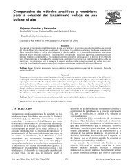
FIGURE 1. Geometry of the zipline indicating the coordinates of
the two endpoints at (0,0) and ( XY , ) , of the rider of mass M at
( xr, y r)
, and of arbitrary points ( xy , ) and ( x, y ) along the line to
the left and right of the rider, respectively. The particular case
plotted here is for parameters i 45 and f 10 (before the
rider mounts the line), 1 (i.e., the rider has the same total mass
as the zipline), L 1 (i.e., the zipline has unit length), and
f 0.25 (i.e, the rider is located a quarter of the way along the
length of the cable). As explained in Sec. III, the zipline has the
shape of one catenary between points (0,0) and
another catenary between ( xr, y r)
and ( XY , ) .
( xr, y r)
, and
Now consider the segment of the cable extending from the
origin to the point ( xy , ) a distance along it. (Assume
fL so that the segment does not include the rider.)
There are three forces on this segment: the tensions T 0 and T
at its two ends, pulling tangential to the line (i.e., at angles
0 and ), and the segment’s weight mg / L . The line is
always in equilibrium, assuming the rider traverses it
slowly. 1 In that case, the three forces must balance. For their
x components, that implies
T0cos0 T cos .
(1)
Therefore the product of the tension and the cosine of the
angle has some constant value K along the cable. To rewrite
it as a dimensionless constant, define b mg / K , so that
T cos mg / b .
(2)
Similarly, balancing the y components of the forces on the
segment implies
T0sin 0 T sin mg . (3)
L
Next, divide Eq. (3) by (2) —or alternatively by Eq. (1)— to
eliminate the tensions and obtain
tan 0 tan b .
(4)
L
Defining another dimensionless constant a tan 0 and a
dimensionless variable u / L , Eq. (4) becomes
tan a bu .
(5)
The coordinates of the rider can be found by dividing the
cable to the left of him into differential pieces of length d .
Integrating the x-components of the length of each piece
gives
fL
xr dl cos .
(6)
0
Divide both sides of this equation by the total length L of the
cable to obtain the normalized x-coordinate of the rider as
f
x du cos .
(7)
0
Substituting Eq. (5) into the identity
2 1/2
cos 1/ sec (1 tan ) , the integral in Eq. (7) can
be performed to obtain the natural logarithm
2
1 a 1 a
ln .
b 2
a bf 1 ( a bf )
1
Here “slowly” means the rider’s acceleration is negligible and his speed
is always much less than the speed of even the slowest transverse waves on
the zipline, i.e., Tmin L / m where T min is the tension in the cable at
the point where it makes the smallest angle relative to the horizontal,
rider,
sin
y , can be obtained by replacing cos with
2 1/2
(1 cos ) in Eq. (7), and the resulting integral
according to Eq. (1). This idea of slowness is analogous to the requirement
that the speed of a piston in a gas-filled cylinder must always be much less
than the speed of sound of the gas if the compressions are to be considered
quasistatic.
this time gives
Lat. Am. J. Phys. Educ. Vol. 5, No. 1, March 2011 6 http://www.lajpe.org
x
If there is no rider on the zipline, then this relation is valid
along its entire length, in which case f 1.
Then defining
X X / L , Eq. (8) becomes
2
0 1 0
1 a a
X ln ,
b a b a b
0 2
0 0 1 ( 0 0 )
where zero subscripts were added to the two constants a and
b to indicate that these are their values when the rider has
zero mass. Similarly, the normalized y-coordinate of the
(8)
(9)

y
2 2
1 a 1 ( a bf )
b
.
(10)
Again, with no rider on the line, put f
obtain
1 and Y Y / L to
Y
2 2
0 0 0
1 a 1 ( a b )
b
0
.
(11)
Equations (9) and (11) cannot be analytically inverted to find
a 0 and b 0 in terms of X and Y . So rather than spelling out
the solution to the problem in terms of the position ( XY , ) of
the right-hand end of the cable, it makes more sense to write
it in terms of the angles i and f that the cable makes at its
two ends without a rider. 2 Recalling the definition of a and
solving Eq. (4) for b, one can write
a and b 0 tan i tan f . (12)
0 tan i
Then the (normalized) position of the right end of the cable
can be determined from Eqs. (9) and (11). That position
remains fixed as the rider mounts the cable, as does the
length of the cable. But the values of a and b change and are
no longer equal to a 0 and b 0 , because the shape (and hence
the two end angles) of the cable change with a rider present.
In fact, it is clear that even for a fixed (nonzero) rider mass,
the values of these two parameters vary as the person
changes position f along the zipline. So the problem now
becomes one of finding the values of a and b for a given
rider position f and mass M (expressed in normalized form as
M / m relative to the cable’s mass). The key to solving
this problem is that Eqs. (8) and (10) give the position ( xy , )
of the cable at the rider’s position relative to the left-hand
end of the cable (in terms of the unknowns a and b). Similar
equations (in terms of the same two unknowns) give the
position ( x, y ) of the right-hand end of the cable relative to
the rider. 3 By imposing the constraints x x X and
y y Y , two equations are obtained in the two unknowns
and a root-finding algorithm can be used to solve for a and b.
The first step is to find the angle 0 of the cable
immediately to the right of the rider. For this purpose,
consider a segment of the cable that starts at the origin and
just barely extends beyond the rider’s point of attachment.
Equation (3) can be modified in this case by adding the
rider’s weight Mg to the right-hand side,
T0 sin 0 T0 sin 0 mgf Mg , (13)
Traveling along a zipline
where became the rider’s position fL, angle became
0 , and likewise for the tension T. Again divide this
equation by Eq. (2) to get
tan 0 tan 0 bf b .
(14)
Consequently the parameter corresponding to a for the righthand
segment of the cable is
a a bf b .
(15)
Unlike Eq. (3), however, Eq. (1) remains valid even when
the point ( xy , ) in Fig. 1 is moved to the right of the rider,
because the rider’s gravitational force does not have an x
component. Thus K has the same value on the left-hand and
right-hand segments of the zipline. Therefore the parameter
corresponding to b for the right-hand segment is unchanged,
b b. Finally, the sum of the lengths of the left-hand and
right-hand segments of the cable must be L, and thus the
parameter corresponding to f for the right-hand segment
must be f 1 f . Now simply substitute these values of
a , b , and f in place of a, b, and f in Eqs. (8) and (10) to
get
and
x
y
2
1 a bf b 1 ( a bf b )
ln ,
b 2
a b b 1 ( a b b)
2 2
1 ( a bf b ) 1 ( a b b)
b
.
(16)
(17)
The sum of Eqs. (8) and (16) is set equal to Eq. (9), and the
sum of Eqs. (10) and (17) to Eq. (11) and the command
―FindRoot‖ in Mathematica is used to solve for a and b for
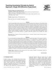
given values of and f. Figure 2 plots the results for equal
to 0, 0.1, 0.5, 1, 2, and ∞ with f varying from 0 to 1 in steps
of 0.01. As explained next, these trajectories interpolate
between a catenary and an ellipse as increases in value.
2
Note that the angle anywhere along the cable (including its two ends),
with or without a (finite-mass) rider, is limited to the range 90 90
since the line can never become vertical according to Eq. (2). Within that
range, tan is always finite and is a single-valued function of .
FIGURE 2. Trajectories followed by the rider through space for six
3
Hereafter, primes are consistently used to indicate parameters of the cable different values of (ratio of the masses of the rider and of the
segment to the right of the rider that correspond to the unprimed parameters
of the cable segment to his left.
zipline) indicated in the legend, for parameters i 45 ,
Lat. Am. J. Phys. Educ. Vol. 5, No. 1, March 2011 7 http://www.lajpe.org

Carl E. Mungan and Trevor C. Lipscombe
f 10 , and L 1 so that X 0.898389 and Y 0.339010 .
The limiting cases are 0 for which the trajectory is a catenary,
and for which the trajectory is an ellipse, as explained in
Sec. III. (For the case of , there are short vertical segments at
the two ends of the trajectory, whose lengths are determined by
requiring the zipline to tauten when the rider clips on.) Do not
confuse these trajectories of the rider with the shapes of the zipline
for a fixed position of the rider (as shown in Fig. 1 for example).
III. SHAPE OF ANY PIECE OF THE CABLE
THAT DOES NOT INCLUDE THE RIDER
Equation (8) can be inverted to obtain f in terms of x . That
expression can then be substituted into Eq. (10) to obtain
y
1
2
a cosh ln a 1
2
a bx
b
.
(18)
Therefore, any piece of the cable that does not include the
rider’s point of attachment is a catenary [8]. An alternative
way to derive this result is to rewrite Eq. (5) as
dy / dx a b / L , differentiate both sides of it with respect
2 1/2
to x, substitute d / dx (1 [ dy / dx ] ) , and finally switch
to normalized coordinates to obtain
2
d y dy
b 1 .
2
dx
dx
2
(19)
By defining z dy / dx with z0a, Eq. (19) can be
integrated twice to get Eq. (18).
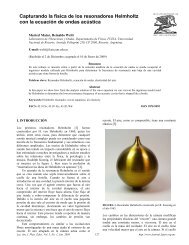
For example, suppose a a 0 and b b 0 as given by Eq.
(12). Then Fig. 3 is a plot of Eq. (18) for a unit length of the
cable making angles i 30 and f 0 at its two ends.
The initial end is at the origin and the final end is at position
( XY , ) given by Eqs. (9) and (11).
FIGURE 3. Shape of a rider-free zipline (of unit length L 1)
when the angles the line makes (relative to the horizontal) at its two
ends (indicated by the black dots) are i 30 and f 0 . The
curve is a portion of a hyperbolic cosine whose minimum is at the
right-hand endpoint, where X 0.951427 and Y 0.267949 .
If the rider is much heavier than the cable, then the
tension in the zipline gets very large and hence b 0 . In
that limit, Eq. (18) reduces to simply y ax . In other words,
the cable consists of one straight segment from the origin to
the rider and a second straight segment from the rider to the
right-hand end. For any given value of f, the rider’s
coordinates can then be determined from the constraint that
the total length of the cable is L. Since the rider moves such
that the sum of his distances to the two endpoints is fixed, he
travels along an elliptical trajectory through space. In
contrast, if the rider is much lighter than the cable, then he
hardly distorts its shape and his trajectory is consequently the
catenary described by Eq. (18).
IV. CONCLUSIONS
Traditionally, the problem in a mechanics course of a
hanging cable consists in finding its shape, both theoretically
and experimentally, under a variety of different conditions
including some novel ones [9–11]. The present paper instead
computes the distortion in a zipline as a weight slowly
moves along its length. As that traveling mass increases from
zero to infinity, the trajectory is found to interpolate between
a hyperbolic cosine and an ellipse, as plotted in Fig. 2.
Instructors or students eager to quickly reproduce that figure
merely have to set the sum of Eqs. (8) and (16) to Eq. (9),
and the sum of Eqs. (10) and (17) to Eq. (11), then use a
numerical solver to find the values of a and b (for any given f
and ). Armed with these values, one can immediately plot
( xy , ) as f is varied from 0 to 1 for fixed .
Remarkably, no numerical technique other than finding
the simultaneous roots of a pair of algebraic equations is
needed to compute these trajectories. Thus this problem is
appropriate for the intermediate classical mechanics course
(traditionally taken in the sophomore or junior undergraduate
years of the physics major). It would make an interesting
student project to actually measure the coordinates of a
hanging weight placed at various positions along a
suspended cable and compare it to the present theoretical
results. In addition to extending familiar variational ideas,
the loaded zipline has importance as a physical model of
curved space. Further, the results here could be of interest to
actual users of ziplines who wish to safely clear obstacles.
REFERENCES
[1] O’Keefe, R., A circular catenary, Am. J. Phys. 64, 660–
661 (1996).
[2] Fallis, M.C., Hanging shapes of nonuniform cables, Am.
J. Phys. 65, 117–122 (1997).
[3] Gruber, R. P., Gruber, A. D., Hamilton, R. and Matthews,
S. M., Space curvature and the “heavy banana paradox”,
Phys. Teach. 29, 147–149 (1991).
[4] Ellingson, J. G., The deflection of light by the Sun due to
three-space curvature, Am. J. Phys. 55, 759–760 (1987).
Lat. Am. J. Phys. Educ. Vol. 5, No. 1, March 2011 8 http://www.lajpe.org

[5] Meckler, A., The hanging string as a model of metric
distortion, Am. J. Phys. 44, 845–850 (1976).
[6] White, G. D. and Walker, M., The shape of “the
Spandex” and orbits upon its surface, Am. J. Phys. 70, 48–
52 (2002).
[7] Zapolsky, H. S., A simple solution of the center loaded
catenary, Am. J. Phys. 58, 1110–1112 (1990).
[8] Nedev, S., The catenary—An ancient problem on the
computer screen, Eur. J. Phys. 21, 451–457 (2000).
Traveling along a zipline
[9] Behroozi, F., Mohazzabi, P. and McCrickard, J. P.,
Remarkable shapes of a catenary under the effect of gravity
and surface tension, Am. J. Phys. 62, 1121–1128 (1994).
[10] Silverman, M. P., Strange, W. and Lipscombe, T. C.,
„String theory‟: Equilibrium configurations of a helicoseir,
Eur. J. Phys. 19, 379–387 (1998).
[11] Mareno, A. and English, L. Q., The stability of the
catenary shapes for a hanging cable of unspecified length,
Eur. J. Phys. 30, 97–108 (2009).
Lat. Am. J. Phys. Educ. Vol. 5, No. 1, March 2011 9 http://www.lajpe.org