Traveling along a zipline

Carl E. Mungan and Trevor C. Lipscombe
f 10 , and L 1 so that X 0.898389 and Y 0.339010 .
The limiting cases are 0 for which the trajectory is a catenary,
and for which the trajectory is an ellipse, as explained in
Sec. III. (For the case of , there are short vertical segments at
the two ends of the trajectory, whose lengths are determined by
requiring the zipline to tauten when the rider clips on.) Do not
confuse these trajectories of the rider with the shapes of the zipline
for a fixed position of the rider (as shown in Fig. 1 for example).
III. SHAPE OF ANY PIECE OF THE CABLE
THAT DOES NOT INCLUDE THE RIDER
Equation (8) can be inverted to obtain f in terms of x . That
expression can then be substituted into Eq. (10) to obtain
y
1
2
a cosh ln a 1
2
a bx
b
.
(18)
Therefore, any piece of the cable that does not include the
rider’s point of attachment is a catenary [8]. An alternative
way to derive this result is to rewrite Eq. (5) as
dy / dx a b / L , differentiate both sides of it with respect
2 1/2
to x, substitute d / dx (1 [ dy / dx ] ) , and finally switch
to normalized coordinates to obtain
2
d y dy
b 1 .
2
dx
dx
2
(19)
By defining z dy / dx with z0a, Eq. (19) can be
integrated twice to get Eq. (18).
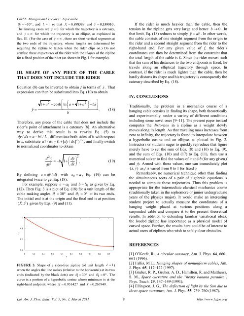
For example, suppose a a 0 and b b 0 as given by Eq.
(12). Then Fig. 3 is a plot of Eq. (18) for a unit length of the
cable making angles i 30 and f 0 at its two ends.
The initial end is at the origin and the final end is at position
( XY , ) given by Eqs. (9) and (11).
FIGURE 3. Shape of a rider-free zipline (of unit length L 1)
when the angles the line makes (relative to the horizontal) at its two
ends (indicated by the black dots) are i 30 and f 0 . The
curve is a portion of a hyperbolic cosine whose minimum is at the
right-hand endpoint, where X 0.951427 and Y 0.267949 .
If the rider is much heavier than the cable, then the
tension in the zipline gets very large and hence b 0 . In
that limit, Eq. (18) reduces to simply y ax . In other words,
the cable consists of one straight segment from the origin to
the rider and a second straight segment from the rider to the
right-hand end. For any given value of f, the rider’s
coordinates can then be determined from the constraint that
the total length of the cable is L. Since the rider moves such
that the sum of his distances to the two endpoints is fixed, he
travels along an elliptical trajectory through space. In
contrast, if the rider is much lighter than the cable, then he
hardly distorts its shape and his trajectory is consequently the
catenary described by Eq. (18).
IV. CONCLUSIONS
Traditionally, the problem in a mechanics course of a
hanging cable consists in finding its shape, both theoretically
and experimentally, under a variety of different conditions
including some novel ones [9–11]. The present paper instead
computes the distortion in a zipline as a weight slowly
moves along its length. As that traveling mass increases from
zero to infinity, the trajectory is found to interpolate between
a hyperbolic cosine and an ellipse, as plotted in Fig. 2.
Instructors or students eager to quickly reproduce that figure
merely have to set the sum of Eqs. (8) and (16) to Eq. (9),
and the sum of Eqs. (10) and (17) to Eq. (11), then use a
numerical solver to find the values of a and b (for any given f
and ). Armed with these values, one can immediately plot
( xy , ) as f is varied from 0 to 1 for fixed .
Remarkably, no numerical technique other than finding
the simultaneous roots of a pair of algebraic equations is
needed to compute these trajectories. Thus this problem is
appropriate for the intermediate classical mechanics course
(traditionally taken in the sophomore or junior undergraduate
years of the physics major). It would make an interesting
student project to actually measure the coordinates of a
hanging weight placed at various positions along a
suspended cable and compare it to the present theoretical
results. In addition to extending familiar variational ideas,
the loaded zipline has importance as a physical model of
curved space. Further, the results here could be of interest to
actual users of ziplines who wish to safely clear obstacles.
REFERENCES
[1] O’Keefe, R., A circular catenary, Am. J. Phys. 64, 660–
661 (1996).
[2] Fallis, M.C., Hanging shapes of nonuniform cables, Am.
J. Phys. 65, 117–122 (1997).
[3] Gruber, R. P., Gruber, A. D., Hamilton, R. and Matthews,
S. M., Space curvature and the “heavy banana paradox”,
Phys. Teach. 29, 147–149 (1991).
[4] Ellingson, J. G., The deflection of light by the Sun due to
three-space curvature, Am. J. Phys. 55, 759–760 (1987).
Lat. Am. J. Phys. Educ. Vol. 5, No. 1, March 2011 8 http://www.lajpe.org