Traveling along a zipline

More documents

Recommendations

Info

$Single Slit Diffraction Experiment - Latin-American Journal of ...$

Carl E. Mungan and Trevor C. Lipscombe The cable bows downward in smooth curves to the left and right of the person, but there will be a cusp in the zipline at the person’s position [7], as illustrated in Fig. 1. At any point ( xy , ) along the cable, the line to the right of that point makes angle relative to the +x axis. In particular, the zipline makes angle 0 at the end attached to the origin. FIGURE 1. Geometry of the zipline indicating the coordinates of the two endpoints at (0,0) and ( XY , ) , of the rider of mass M at ( xr, y r) , and of arbitrary points ( xy , ) and ( x, y ) along the line to the left and right of the rider, respectively. The particular case plotted here is for parameters i 45 and f 10 (before the rider mounts the line), 1 (i.e., the rider has the same total mass as the zipline), L 1 (i.e., the zipline has unit length), and f 0.25 (i.e, the rider is located a quarter of the way along the length of the cable). As explained in Sec. III, the zipline has the shape of one catenary between points (0,0) and another catenary between ( xr, y r) and ( XY , ) . ( xr, y r) , and Now consider the segment of the cable extending from the origin to the point ( xy , ) a distance along it. (Assume fL so that the segment does not include the rider.) There are three forces on this segment: the tensions T 0 and T at its two ends, pulling tangential to the line (i.e., at angles 0 and ), and the segment’s weight mg / L . The line is always in equilibrium, assuming the rider traverses it slowly. 1 In that case, the three forces must balance. For their x components, that implies T0cos0 T cos . (1) Therefore the product of the tension and the cosine of the angle has some constant value K along the cable. To rewrite it as a dimensionless constant, define b mg / K , so that T cos mg / b . (2) Similarly, balancing the y components of the forces on the segment implies T0sin 0 T sin mg . (3) L Next, divide Eq. (3) by (2) —or alternatively by Eq. (1)— to eliminate the tensions and obtain tan 0 tan b . (4) L Defining another dimensionless constant a tan 0 and a dimensionless variable u / L , Eq. (4) becomes tan a bu . (5) The coordinates of the rider can be found by dividing the cable to the left of him into differential pieces of length d . Integrating the x-components of the length of each piece gives fL xr dl cos . (6) 0 Divide both sides of this equation by the total length L of the cable to obtain the normalized x-coordinate of the rider as f x du cos . (7) 0 Substituting Eq. (5) into the identity 2 1/2 cos 1/ sec (1 tan ) , the integral in Eq. (7) can be performed to obtain the natural logarithm 2 1 a 1 a ln . b 2 a bf 1 ( a bf ) 1 Here “slowly” means the rider’s acceleration is negligible and his speed is always much less than the speed of even the slowest transverse waves on the zipline, i.e., Tmin L / m where T min is the tension in the cable at the point where it makes the smallest angle relative to the horizontal, rider, sin y , can be obtained by replacing cos with 2 1/2 (1 cos ) in Eq. (7), and the resulting integral according to Eq. (1). This idea of slowness is analogous to the requirement that the speed of a piston in a gas-filled cylinder must always be much less than the speed of sound of the gas if the compressions are to be considered quasistatic. this time gives Lat. Am. J. Phys. Educ. Vol. 5, No. 1, March 2011 6 http://www.lajpe.org x If there is no rider on the zipline, then this relation is valid along its entire length, in which case f 1. Then defining X X / L , Eq. (8) becomes 2 0 1 0 1 a a X ln , b a b a b 0 2 0 0 1 ( 0 0 ) where zero subscripts were added to the two constants a and b to indicate that these are their values when the rider has zero mass. Similarly, the normalized y-coordinate of the (8) (9)
y 2 2 1 a 1 ( a bf ) b . (10) Again, with no rider on the line, put f obtain 1 and Y Y / L to Y 2 2 0 0 0 1 a 1 ( a b ) b 0 . (11) Equations (9) and (11) cannot be analytically inverted to find a 0 and b 0 in terms of X and Y . So rather than spelling out the solution to the problem in terms of the position ( XY , ) of the right-hand end of the cable, it makes more sense to write it in terms of the angles i and f that the cable makes at its two ends without a rider. 2 Recalling the definition of a and solving Eq. (4) for b, one can write a and b 0 tan i tan f . (12) 0 tan i Then the (normalized) position of the right end of the cable can be determined from Eqs. (9) and (11). That position remains fixed as the rider mounts the cable, as does the length of the cable. But the values of a and b change and are no longer equal to a 0 and b 0 , because the shape (and hence the two end angles) of the cable change with a rider present. In fact, it is clear that even for a fixed (nonzero) rider mass, the values of these two parameters vary as the person changes position f along the zipline. So the problem now becomes one of finding the values of a and b for a given rider position f and mass M (expressed in normalized form as M / m relative to the cable’s mass). The key to solving this problem is that Eqs. (8) and (10) give the position ( xy , ) of the cable at the rider’s position relative to the left-hand end of the cable (in terms of the unknowns a and b). Similar equations (in terms of the same two unknowns) give the position ( x, y ) of the right-hand end of the cable relative to the rider. 3 By imposing the constraints x x X and y y Y , two equations are obtained in the two unknowns and a root-finding algorithm can be used to solve for a and b. The first step is to find the angle 0 of the cable immediately to the right of the rider. For this purpose, consider a segment of the cable that starts at the origin and just barely extends beyond the rider’s point of attachment. Equation (3) can be modified in this case by adding the rider’s weight Mg to the right-hand side, T0 sin 0 T0 sin 0 mgf Mg , (13) Traveling along a zipline where became the rider’s position fL, angle became 0 , and likewise for the tension T. Again divide this equation by Eq. (2) to get tan 0 tan 0 bf b . (14) Consequently the parameter corresponding to a for the righthand segment of the cable is a a bf b . (15) Unlike Eq. (3), however, Eq. (1) remains valid even when the point ( xy , ) in Fig. 1 is moved to the right of the rider, because the rider’s gravitational force does not have an x component. Thus K has the same value on the left-hand and right-hand segments of the zipline. Therefore the parameter corresponding to b for the right-hand segment is unchanged, b b. Finally, the sum of the lengths of the left-hand and right-hand segments of the cable must be L, and thus the parameter corresponding to f for the right-hand segment must be f 1 f . Now simply substitute these values of a , b , and f in place of a, b, and f in Eqs. (8) and (10) to get and x y 2 1 a bf b 1 ( a bf b ) ln , b 2 a b b 1 ( a b b) 2 2 1 ( a bf b ) 1 ( a b b) b . (16) (17) The sum of Eqs. (8) and (16) is set equal to Eq. (9), and the sum of Eqs. (10) and (17) to Eq. 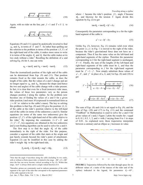(11) and the command ―FindRoot‖ in Mathematica is used to solve for a and b for given values of and f. Figure 2 plots the results for equal to 0, 0.1, 0.5, 1, 2, and ∞ with f varying from 0 to 1 in steps of 0.01. As explained next, these trajectories interpolate between a catenary and an ellipse as increases in value. 2 Note that the angle anywhere along the cable (including its two ends), with or without a (finite-mass) rider, is limited to the range 90 90 since the line can never become vertical according to Eq. (2). Within that range, tan is always finite and is a single-valued function of . FIGURE 2. Trajectories followed by the rider through space for six 3 Hereafter, primes are consistently used to indicate parameters of the cable different values of (ratio of the masses of the rider and of the segment to the right of the rider that correspond to the unprimed parameters of the cable segment to his left. zipline) indicated in the legend, for parameters i 45 , Lat. Am. J. Phys. Educ. Vol. 5, No. 1, March 2011 7 http://www.lajpe.org
Page 1: Traveling along a zipline Carl E. M
Page 5: [5] Meckler, A., The hanging string

Traveling along a zipline

You also want an ePaper? Increase the reach of your titles

Delete template?

Save as template?