Download PDF - Ivie

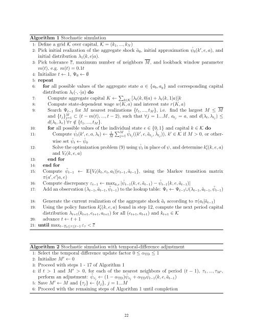
Algorithm 1 Stochastic simulation
1: Define a grid K over capital, K = (k 1 , ..., k N )
2: Pick initial realization of the aggregate shock ã 0 , initial approximation ˆψ 0 (k ′ , e, a), and
initial distribution λ 1 (k, e|a).
3: Pick tolerance ε, maximum number of neighbors M, and lookback window parameter
m(t), e.g. m(t) = 0.1t
4: Initialize t ← 1, Ψ 0 ← ∅
5: repeat
6: for all possible values of the aggregate state a ∈ {a b , a g } and corresponding capital
distribution λ t (·, ·|a) do
7: Compute aggregate capital K ← ∑ k∈K [λ t(k, 0|a) + λ t (k, 1|a)]k
8: Compute state-dependent wage w(K, a) and interest rate r(K, a)
9: Search Ψ t−1 for M nearest realizations {t 1 , ..., t M }, i.e. find the largest M ≤ M
and {t j } M j=1 ⊂ (t − m(t), ..., t − 2), such that ∀j = 1...M, a tj = a, and d(λ t , λ tj ) ≤
d(λ t , λ τ ) ∀τ /∈ {t 1 , ..., t M }.
10: for all possible values of the individual state e ∈ {0, 1} and capital k ∈ K do
11: Compute ˆψ ∑
t (k ′ , e, a, λ t ) ← 1 M ˜ψ M j=1 tj ((k ′ , e, ã tj , ˜λ tj )), k ′ ∈ K if M > 0, or otherwise
set ˆψ t ← ˆψ 0
12: Solve the optimization problem (9) using ˆψ t in place of ψ, and determine k t(k, ′ e, a)
and V t (k, e, a)
13: end for
14: end for
15: Compute ˜ψ t−1 ← E{V t (k t , e t , a t )|e t−1 , ã t−1 }, using the Markov transition matrix
π(a ′ , e ′ |a, e)
16: Compute discrepancy ε t−1 ← max k,e | ˆψ t−1 (k, e, ã t−1 ) − ˜ψ t−1 (k, e, ã t−1 )|
17: Add an observation (λ t−1 , ã t−1 , ˜ψ t−1 ) to the lookup table: Ψ t ← Ψ t−1 ∪(λ t−1 , ã t−1 , ˜ψ t−1 )
18: Generate the current realization of the aggregate shock ã t according to π(a t |ã t−1 )
19: Using the policy function k t(k, ′ e, a) found in step 12, compute the next period capital
distribution λ t+1 (k t+1 , e t+1 , a t+1 ) for all (e t+1 , a t+1 ) and k t+1 ∈ K
20: advance t ← t + 1
21: until max t−T0 ≤τ≤t−1 ε τ < ε
Algorithm 2 Stochastic simulation with temporal-difference adjustment
1: Select the temporal difference update factor 0 ≤ α TD ≤ 1
2: Initialize M ′ ← 0
3: Proceed with steps 1 - 17 of Algorithm 1
4: if t > 1 and M ′ > 0, for each of the nearest neighbors of period (t − 1), τ 1 , ..., τ M ′,
perform an adjustment: ˜ψτj ← (1 − α TD ) ˜ψ τj + α TD ˜ψt−1 (k, e, ã t−1 )
5: Save M ′ ← M and {τ j } ← {t j }, j = 1...M
6: Proceed with the remaining steps of Algorithm 1 until completion
20
22