GROEBNER BASIS CONVERSION USING THE FGLM ALGORITHM ...

GROEBNER BASIS CONVERSION USING THE FGLM
ALGORITHM
PHILIP BENGE, VALERIE BURKS, NICHOLAS COBAR
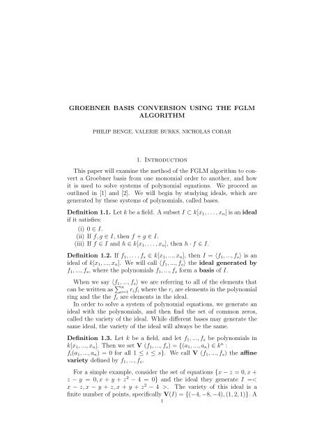
1. Introduction
This paper will examine the method of the FGLM algorithm to convert
a Groebner basis from one monomial order to another, and how
it is used to solve systems of polynomial equations. We proceed as
outlined in [1] and [2]. We will begin by studying ideals, which are
generated by these systems of polynomials, called bases.
Definition 1.1. Let k be a field. A subset I ⊂ k[x1,...,xn] is an ideal
if it satisfies:
(i) 0 ∈ I.
(ii) If f,g ∈ I, then f + g ∈ I.
(iii) If f ∈ I and h ∈ k[x1,...,xn], then h · f ∈ I.
Definition 1.2. If f1,...,fs ∈ k[x1,...,xn], then I = 〈f1,...,fs〉 is an
ideal of k[x1,...,xn]. We will call 〈f1,...,fs〉 the ideal generated by
f1,...,fs, where the polynomials f1,...,fs form a basis of I.
When we say 〈f1,...,fs〉 we are referring to all of the elements that
can be written as �n i=1 rifi where the ri are elements in the polynomial
ring and the the fi are elements in the ideal.
In order to solve a system of polynomial equations, we generate an
ideal with the polynomials, and then find the set of common zeros,
called the variety of the ideal. While different bases may generate the
same ideal, the variety of the ideal will always be the same.
Definition 1.3. Let k be a field, and let f1,...,fs be polynomials in
k[x1,...,xn]. Then we set V (f1,...,fs) = {(a1,...,an) ∈ k n :
fi(a1,...,an) = 0 for all 1 ≤ i ≤ s}. We call V (f1,...,fs) the affine
variety defined by f1,...,fs.
For a simple example, consider the set of equations {x − z = 0,x +
z − y = 0,x + y + z 2 − 4 = 0} and the ideal they generate I =<
x − z,x − y + z,x + y + z 2 − 4 >. The variety of this ideal is a
finite number of points, specifically V(I) = {(−4, −8, −4), (1, 2, 1)}. A
1

2 PHILIP BENGE, VALERIE BURKS, NICHOLAS COBAR
variety does not have to be a finite set of points, but if it is, the ideal
is called zero-dimensional.
In order to study these ideals and their bases, a standard must be
set for the way in which the polynomials are written. This is essential
because the division algorithm, which is associative in single variable
calculations, is not associative when multiple variables are involved.
Also, what would constitute a Groebner basis under one monomial
order would not necessarily be the same under another.
Definition 1.4. A monomial ordering on k[x1,...,xn] is any relation
> on Z n ≥0, or equivalently, any relation on the set of monomials
x α ,α ∈ Z n ≥0, satisfying:
(1) > is a total (or linear) ordering on Z n ≥0.
(2) If α > β and γ ∈ Z n ≥0, then α + γ > β + γ.
(3) > is a well-ordering on Z n ≥0. This means that every nonempty
subset of Z n ≥0 has a smallest element under >.
Within polynomials, the monomials are generally written in descending
order. Within the monomial itself, individual variables are also
written in descending order with x1 > x2 > ... > xn. To determine
precedence under a monomial ordering, the exponents of the variables
in a monomial are written as an ordered n-tuple to allow the reader to
find the vector difference. An example of each type of monomial ordering
will be given using the monomials x1x 2 2 and x 3 2x 4 3. The n-tuples
for these monomials (represented by α and β) are α = (1, 2, 0) and
β = (0, 3, 4), respectively.
Three commonly used monomial orders are lexicographic, graded
lexicographic, and graded reverse lexicographic. In lexicographic order,
or lex, a monomial with degree α is greater than another monomial with
degree β if and only if the left-most, non-zero component of α − β is
greater than 0. In graded lexicographic, or grlex, the monomial with
the higher total degree is greater than the other. If the monomials’
degrees are equal, then we use lex to break the tie. Finally, graded
reverse lexicographic, also called grevlex, is exactly like grlex in that
it first compares the degrees of the monomials, and the one with the
higher degree is taken to be greater. However, in the event of equal
degrees, it does not revert back to lex ordering to break ties. Instead a
monomial with degree α is greater than another monomial with degree
β if the right-most, non-zero component of α − β is less than 0.
Example 1.5.
(1) x1x 2 2 >lex x 3 2x 4 3 since α − β = (1, −1, −4).
(2) x1x 2 2

GROEBNER BASIS CONVERSION USING THE FGLM ALGORITHM 3
(3) x1x 2 2
be a monomial order. Then the multidegree of f is multideg(f) =
max{α ∈ Zn ≥0 : aα �= 0} (the maximum is taken with respect to >).
The leading coefficient of f is LC(f) = amultideg(f) ∈ k, and the
leading monomial of f is LM(f) = xmultideg(f) (with coefficient 1).
The leading term of f is LT(f) = LC(f) · LM(f). For example, if
f = 3x3y2 − x3y + x2 − y, then multideg(f) = (3, 2, 0), LC(f) = 3,
LM(f) = x3y2 , and the LT(f) = 3x3y2 with respect to lexicographic
order.
Definition 1.6. Fix a monomial order. A finite subset G = {g1,...,gt}
of an ideal I is said to be a Groebner basis if
< LT(g1),...,LT(gt) > = < LT(I) >. A Groebner basis is call reduced
if
(1) LC(p) = 1 for all p ∈ G.
(2) For all p ∈ G, no monomial of p lies in 〈LT(G − {p})〉.
This means that the leading term of any element of I must be divisible
by one of the LT(gi) for G to be a Groebner basis. To divide
polynomials we use the following division algorithm:
Definition 1.7. Fix a monomial order > on Z n ≥0, and let F = (f1,...,fs)
be an ordered s-tuple of polynomials in k[x1,...,xn]. Then every
f ∈ k[x1,...,xn] can be written as
f = a1f1 + ... + asfs + r,
where ai,r ∈ k[x1,...,xn], and either r = 0 or r is a linear combination,
with coefficients in k, of monomials, none of which is divisible by any
of LT(f1),...,LT(fs). We will call r a remainder of f on division by
F. Furthermore if ai,fi �= 0, then we have
multideg(f) ≥ multideg(aifi).
For example, consider the ideal I =< x 2 + y 2 + z 2 − 2x,x 3 − yz −
x,x − y + 2z >. Take the monomial order graded lexicographic. Then
a Groebner basis, G, for I is G = {x − y + 2z, 2y 2 − 4yz + 5z 2 − 2y +
4z, 3yz 2 + 4z 3 − 10yz + 11z 2 , 375z 4 + 974z 3 − 1460yz + 144z 2 }.
Groebner bases have some very useful properties. In the case of
determining if a function f ∈ k[x1,...,xn] is in an ideal, I, simply
divide f by a Groebner basis for I and then f ∈ I if and only if the
remainder is zero. For example, let I and G be as stated above, and

4 PHILIP BENGE, VALERIE BURKS, NICHOLAS COBAR
f = 14xy − 2z + 3. Then dividing f by G = {g1,g2,g3,g4} using
the division algorithm yields f = 14y · g1 + 7 · g2 + r, where r =
−35z 2 + 14y − 30z + 3. Since r �= 0, f /∈ I.
We would like to mention that a reduced Groebner basis is unique
with respect to a monomial ordering, and from that, two ideals are
equal if and only if their reduced Groebner bases with respect to a
monomial ordering are equal.
We note that an ideal I is zero-dimensional if and only if it satisfies
the following criteria:
Theorem 1.8. Let V=V(I) be an affine variety in Cn and fix a monomial
ordering in C[x1,...,xn]. Then the following statements are equivalent:
(1) V is a finite set.
(2) For each i, 1 ≤ i ≤ n, there is some mi ≥ 0 such that x mi
i ∈<
LT(I) >.
(3) Let G be a Groebner basis for I. Then for each i, 1 ≤ i ≤ n,
there is some mi ≥ 0 such that x mi
i = LM(gi) for some gi ∈ G.
(4) The C-vector space S = span(xα : xα /∈< LT(I) >) is finitedimensional.
(5) The C-vector space C[x1,...,xn]/I is finite-dimensional.
The proof of this theorem is non-trivial, however the proof goes
beyond the scope of this paper. As we can see, if we have a zerodimensional
ideal, then for each variable xi, there is a polynomial in
the Groebner basis for I with a power of xi as a leading monomial.
Consider the following example of a zero-dimensional ideal.
Example 1.9. Let I =< xy 3 − x 2 ,x 3 y 2 − y > in R[x,y]. Using grlex
the Groebner basis is G = {x 3 y 2 − y,x 4 − y 2 ,xy 3 − x 2 ,y 4 − xy}
and 〈LT(I)〉 = 〈x 3 y 2 ,x 4 ,xy 3 ,y 4 〉. We can draw a picture in Z 2 ≥0 to
represent the exponent vectors of the monomials in 〈LT(I)〉 and its
complement as follows. The vectors
α(1) = (3, 2),
α(2) = (4, 0),
α(3) = (1, 3),
α(4) = (0, 4)
are the exponent vectors of the generators of 〈LT(I)〉. Thus, the elements
of ((3, 2) + Z 2 ≥0) ∪ ((4, 0) + Z 2 ≥0) ∪ ((1, 3) + Z 2 ≥0) ∪ ((0, 4) + Z 2 ≥0)
are the exponent vectors of monomials in 〈LT(I)〉. As a result, we can
represent the monomials in 〈LT(I)〉 by the integer points in the shaded
region in Z 2 ≥0 shown below in Figure 1.

GROEBNER BASIS CONVERSION USING THE FGLM ALGORITHM 5
Figure 1
2. The FGLM Algorithm
The difficulties that arise from trying to compute reduced Groebner
bases with respect to lex ordering can seem insurmountable and enough
to render Groebner bases useless. Fortunately there exists a way to
circumvent some of the difficulties. The aptly-named FGLM algorithm
was developed by J.C. Faugère, P. Gianni, D. Lazard, and T. Mora.
As mentioned earlier, it allows one to take a Groebner basis from the
relatively easy calculations of a grevlex ordering and convert it to the
reduced Groebner basis for the same ideal with respect to another
monomial ordering. The drawback to this algorithm is that it only
applies to zero-dimensional ideals. This will be explained in a later
section. In the algorithm, we will be converting a non-lex Groebner
basis to lex Groebner basis, but the FGLM algorithm can be used
to convert a Groebner basis from any monomial order to any other
monomial order.
First, of course, one must have an initial Groebner basis, G, with
respect to an initial monomial order. The algorithm then progresses
through three steps for each of the monomials in the ring k[x1,...,xn]
in increasing lex order. At the beginning of each loop, there will be two
sets: Glex, which is initially empty but will become the new Groebner
basis for the desired monomial order, and Blex, which is also initially
empty but will grow to be the lex monomial basis of the quotient ring
k[x1,...,xn]/I as a k-vector space.
The FGLM algorithm consists of three main parts.

6 PHILIP BENGE, VALERIE BURKS, NICHOLAS COBAR
(1) Main Loop: For this first step the user will take the current
input monomial x α , initially 1, and find the remainder under
division by G, denoted x αG . Recall that G is the Groebner
basis of the ideal with respect to the original monomial ordering.
There are two possible cases for what will happen to the
remainder. For the first, if x αG is linearly dependent on the
remainders of the other members of Blex, then we have a linear
combination such that
xαG − �
cjxα(j)G = 0
j
where x α(j) ∈ Blex and cj ∈ k. This implies that g = x α −
�
j cjx α(j) ∈ I. So we add g to the list Glex as the last element.
Because we work through the various x α in increasing order
with respect to the new ordering, a polynomial g that is added
to Glex will always have x α with a coefficient of 1 as its leading
term.
In the second case, x αG is linearly independent of the remainders
of the items in Blex. In this event, x α is added to Blex.
If the first case applied and we added a polynomial to Glex,
then Glex must be tested to see if it is the desired Groebner
basis. To do this, we use the Termination Test, the second part
of the FGLM algorithm.
(2) Termination Test: In the event that a new polynomial, g, was
added to Glex, the user must compute LT(g). If LT(g) is a
power of xi, where xi is the greatest variable in the new monomial
ordering, then the algorithm terminates. Otherwise, proceed
to the third part of the algorithm, the Next Monomial
step.
(3) Next Monomial: In this phase of the algorithm, simply replace
the x α that has just been processed with the next monomial
with respect to the new order which is not divisible by any of
the leading terms of the polynomials in Glex.
The user repeats the steps of this algorithm until the conditions are
met for the Termination Test.
Notice that whenever a polynomial g is added to Glex, its leading
term is LT(g) = x α with coefficient 1, hence each basis element must
be monic. Also, because the leading term of each basis element is
linearly independent of the leading terms of all other elements, the
Groebner basis obtained from this algorithm must be reduced. The

GROEBNER BASIS CONVERSION USING THE FGLM ALGORITHM 7
following example fully demonstrates the algorithm for the reader to
clearly see how it works before we present the proof.
3. Example
We will use the FGLM algorithim to find a lexicographic order (with
x > y > z) Groebner basis for the ideal I =< x 2 + 2y 2 − y − 2z,x 2 −
8y 2 +10z−1,x 2 −7yz > from the graded reverse lexicographic Groebner
basis, G = {980z 2 − 18y − 201z + 13, 35yz − 4y + 2z − 1, 10y 2 − y −
12z + 1, 5x 2 − 4y + 2z − 1}. We start with the least variable in the
monomial order, z, and consider it raised to the 0 degree. We then
calculate the remainder of z 0 under division by G. We then continue
increasing the degree of z and finding remainders under division by G
until we find a remainder that is linearly dependent upon the other
remainders. This linearly dependent remainder is subtracted from the
dividend for which it corresponds and this polynomial is added to the
set making up the Groebner basis.
z 0G = 1 G = 1
z G = z
z 2G = 9
490
z 3G = 2817
480200
201 13 y + z − 980 980
y + 26653
960400
z − 2109
960400
Since z 3G is a linear combination of 1 G , z G , and z 2G ,
g1 = z 3 − 313
980 z2 + 37 1
z +
980 490
is the first polynomial added to Glex.
Now we consider the next variable in the monomial order, y. We
again take the remainder with respect to G.
yG = y
We find y itself can be expressed as a linear combination, namely
y = 490
9 z2G − 67
6 zG + 13
18
and subsequently
g2 = y − 490
9 z2 + 67 13
z −
6 18
is added to Glex.
Lastly we consider the greatest variable in the order, x.
x G = x
x2G = 4 2 1 y − z + 5 5 5
Now x2G can be expressed in relation to yG and zG and accordingly
g3 = x 2 − 392
9 z2 + 28 7
z −
3 9

8 PHILIP BENGE, VALERIE BURKS, NICHOLAS COBAR
is the final function added to Glex, leaving us with
Glex = {g1,g2,g3},
our desired lex Groebner basis.
Before we show that the FGLM algorithm is a valid method for
changing the ordering of a Groebner basis, we will state the following
lemma:
Lemma 3.1. (Dickson’s Lemma) Given an infinite list x α(1) ,x α(2) ,...
of monomials in k[x1,...,xn], there is an N ∈ N such that every x α(i)
is divisible by one of x α(1) ,...,x α(N) .
Theorem 3.2. The algorithm described above terminates on every input
Groebner basis, G, that generates a zero-dimensional ideal I, and
correctly computes a lex Groebner basis, Glex, for I and the lex monomial
basis, Blex, for the quotient ring k[x1,...,xn]/I.
Proof. We begin with the key observation that monomials are added
to the list Blex in strictly increasing lex order. Similarly, if Glex =
{g1,...,gk}, then
LT(g1) lex ... >lex xn. We
will prove that Glex is a lex Groebner basis for I by contradiction. Suppose
there were some g ∈ I such that LT(g) is not a multiple of any

GROEBNER BASIS CONVERSION USING THE FGLM ALGORITHM 9
of the LT(gi), i = 1,...,k. Without loss of generality, we may assume
that g is reduced with respect to Glex.
If LT(g) is greater than LT(gk) = x a1
1 , then one easily sees that
LT(g) is a multiple of LT(gk). Hence, this case cannot occur, which
means that
LT(gi) < LT(g) ≤ LT(gi+1)
for some i < k. But recall that the algorithm places monomials into
Blex in strictly increasing order, and the same is true for the LT(gi).
All the non-leading monomials in g must be less than LT(g) in the
lex order. They are not divisible by any of LT(gj) for j ≤ i, since
g is reduced. So, the non-leading monomials that appear in g would
have been included in Blex by the time LT(g) was reached by the Next
Monomial procedure, and g would have been the next polynomial after
gi included in Glex. This contradicts our assumption on g, which proves
that Glex is a lex Groebner basis for I.
To find a monomial basis for k[x1,...,xn]/I, we need to find all
monomials not in 〈LT(g)〉 for all g ∈ Glex. But Blex contains all such
monomials, so Blex forms a monomial basis for the quotient ring as a
k-vector space. So Blex consists of all monomials determined by the
Groebner basis Glex. �
If I were not a zero dimensional ideal, then some monomial would
always yield a linearly independent remainder, and the Main Loop
would never terminate. By Moeller and Mora [3] we know the upperbound,
call it B, of the total degree of a Groebner basis to be
((n + 1)(d + 1) + 1) (n+1)2s+1
where n is the number of variables in the
ideal, d is the total degree of the ideal, and s is the dimension of the
ideal. To assure termination on a positive dimensional ideal, if we know
B, then for each monomial x, the main loop would need only to run
up to x B , and terminate if the loop does not do so before x B . However,
because the upper bound of the total degree grows rapidly as the
dimension of the ideal increases, it is practical to only use the FGLM
algorithm on zero dimensional ideals.
4. Conclusion
Finding Groebner bases with respect to lexicographic order is useful
because of the algorithm’s ability to eliminate the largest term in
at least one of the basis elements which makes solving a system of
polynomial equations much easier. Consider a group of polynomial
equations f1,...,fs. These equations determine I = 〈f1,...,fs〉 and to
solve this system, we want to find V(I). If we compute V(I) using
a lex Groebner basis, then we will get equations g1,...,gt forming the

10 PHILIP BENGE, VALERIE BURKS, NICHOLAS COBAR
Groebner basis. Using the property of lexicographic order mentioned
above, we can then back substitute to find the solutions to the system.
However, finding the lexicographic Groebner basis directly can be computationally
expensive. For example, the lexicographic Groebner basis
for I =< x 5 + y 5 + z 5 − 1,x 3 + y 3 + z 2 − 1 > contains a polynomial
with 415 terms, total degree of 37, with a largest coefficient of
141,592,532,029,352. It is instead more efficient to find a Grobner Basis
with respect to the graded reverse lexicographic order, and then
use the FGLM algorithm to convert the basis to lexicographic order.
The Groebner basis in graded reverse lexicographic order for the above
ideal is considerably less pathological: the largest polynomial has 38
terms, total degree of 11, and the largest coefficient is 7. The FGLM
algorithm allows us to more efficiently compute lexicographic Groebner
bases, which have a wide range of applications.
Acknowledgements
The authors thank Robert Lax for his thought provoking lectures,
Jesse Taylor for helpful discussions concerning this paper, and the VI-
GRE program for our funding.
References
[1] Cox, D., Little, J., and O’Shea, D. (2007). Ideals, Varieties, and Algorithms
(3 rd ed.). New York: Springer.
[2] Cox, D., Little, J., and O’Shea, D. (1998). Using Algebraic Geometry. New
York: Springer.
[3] Moeller, H. M., and Mora, F. (1984). Upper and lower Bound for the degree
of Groebner bases, Lecture Notes in Computer Science, 174, 172-183.