Chapter 4 Line Sweep - TI

Chapter 4
Line Sweep
In this chapter we will discuss a simple and widely applicable paradigm to design geometric
algorithms: the so-called Line-Sweep (or Plane-Sweep) technique. It can be
used to solve a variety of different problems, some examples are listed below. The first
part may come as a reminder to many of you, because you should have heard something
about line-sweep in one of the basic CS courses already. However, we will soon proceed
and encounter a couple of additional twists that were most likely not covered there.
Consider the following geometric problems.
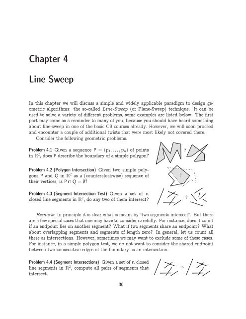
Problem 4.1 Given a sequence P = (p1,...,pn) of points
inR 2 , does P describe the boundary of a simple polygon?
Problem 4.2 (Polygon Intersection) Given two simple polygons
P and Q inR 2 as a (counterclockwise) sequence of
their vertices, is P�Q =�?
Problem 4.3 (Segment Intersection Test) Given a set of n
closed line segments inR 2 , do any two of them intersect?
Remark: In principle it is clear what is meant by “two segments intersect”. But there
are a few special cases that one may have to consider carefully. For instance, does it count
if an endpoint lies on another segment? What if two segments share an endpoint? What
about overlapping segments and segments of length zero? In general, let us count all
these as intersections. However, sometimes we may want to exclude some of these cases.
For instance, in a simple polygon test, we do not want to consider the shared endpoint
between two consecutive edges of the boundary as an intersection.
Problem 4.4 (Segment Intersections) Given a set of n closed
line segments in R 2 , compute all pairs of segments that
intersect.
30
?
⇒
?
?

CG 2012 4.1. Interval Intersections
Problem 4.5 (Segment Arrangement) Given a set ofnclosed
line segments in R 2 , construct the arrangement induced
by S, that is, the subdivision ofR 2 induced by S.
Problem 4.6 (Map Overlay) Given two setsSandT ofnand
m, respectively, pairwise interior disjoint line segments in
R 2 , construct the arrangement induced by S�T.
In the following we will use Problem 4.4 as our flagship example.
Trivial Algorithm. Test all the�n
2�pairs of segments fromSinO(n 2 ) time and O(n) space.
For Problem 4.4 this is worst-case optimal because there may by Ω(n 2 ) intersecting pairs.
But in case that the number of intersecting pairs is, say, linear in n there is still hope
to obtain a subquadratic algorithm. Given that there is a lower bound of Ω(n logn) for
Element Uniqueness (Given x1,...,xn R, is there an i�= j such that xi = xj?) in the
algebraic computation tree model, all we can hope for is an output-sensitive runtime of
the form O(n logn+k), where k denotes the number of intersecting pairs (output size).
4.1 Interval Intersections
As a warmup let us consider the corresponding problem inR 1 .
Problem 4.7 Given a set I of n intervals [ℓi,ri]�R, 1�i�n. Compute all pairs of
intervals from I that intersect.
Theorem 4.8 Problem 4.7 can be solved in O(n logn+k) time and O(n) space, where
k is the number of intersecting pairs from�I
2�.
Proof. First observe that two real intervals intersect if and only if one contains the right
endpoint of the other.
£
Sort the set {(ℓi,0)|1�i�n}�{(ri,1)|1�i�n} in increasing lexicographic order
and denote the resulting sequence by P. Store along with each point from P its origin
(i). Walk through P from start to end while maintaining a list L of intervals that contain
the current point p P.
Whenever p = (ℓi,0), 1�i�n, insert i into L. Whenever p = (ri,1), 1�i�n,
remove i from L and then report for all j L the pair {i,j} as intersecting.
4.2 Segment Intersections
How can we transfer the (optimal) algorithm for the corresponding problem inR 1 to the
plane? InR 1 we moved a point from left to right and at any point resolved the situation
locally around this point. More precisely, at any point during the algorithm, we knew all
31
⇒
⇒

Chapter 4. Line Sweep CG 2012
intersections that are to the left of the current (moving) point. A point can be regarded
a hyperplane inR 1 , and the corresponding object inR 2 is a line.
General idea. Move a line ℓ (so-called sweep line) from left to right over the plane, such
that at any point during this process all intersections to the left of ℓ have been reported.
Sweep line status. The list of intervals containing the current point corresponds to a list L
of segments (sorted by y-coordinate) that intersect the current sweep line ℓ. This list L is
called sweep line status (SLS). Considering the situation locally around L, it is obvious
that only segments that are adjacent in L can intersect each other. This observation
allows to reduce the overall number of intersection tests, as we will see. In order to
allow for efficient insertion and removal of segments, the SLS is usually implemented as
a balanced binary search tree.
Event points. The order of segments in SLS can change at certain points only: whenever
the sweep line moves over a segment endpoint or a point of intersection of two segments
from S. Such a point is referred to as an event point (EP) of the sweep. Therefore we
can reduce the conceptually continuous process of moving the sweep line over the plane
to a discrete process that moves the line from EP to EP. This discretization allows for
an efficient computation.
At any EP several events can happen simultaneously: several segments can start
and/or end and at the same point a couple of other segments can intersect. In fact
the sweep line does not even make a difference between any two event points that have
the same x-coordinate. To properly resolve the order of processing, EPs are considered
in lexicographic order and wherever several events happen at a single point, these are
considered simultaneously as a single EP. In this light, the sweep line is actually not a
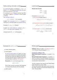
line but an infinitesimal step function (see Figure 4.1).
Event point schedule. In contrast to the one-dimensional situation, in the plane not all
EP are known in advance because the points of intersection are discovered during the
algorithm only. In order to be able to determine the next EP at any time, we use a
priority queue data structure, the so-called event point schedule (EPS).
Along with every EP p store a list end(p) of all segments that end at p, a list begin(p)
of all segments that begin at p, and a list int(p) of all segments in SLS that intersect at
p a segment that is adjacent to it in SLS.
Along with every segment we store pointers to all its appearances in an int(¡) list of
some EP. As a segment appears in such a list only if it intersects one of its neighbors
32

CG 2012 4.2. Segment Intersections
1
2
3
4
5
p
(a) Before.
5
6
3
7
2
1
2
3
4
5
p
(b) After.
Figure 4.1: Handling an event point p. Ending segments are shown red (dashed),
starting segments green (dotted), and passing segments blue (solid).
there, every segment needs to store at most two such pointers.
Invariants.
1. L is the sequence of segments from S that intersect ℓ, ordered by y-coordinate of
their point of intersection.
2. E contains all endpoints of segments from S and all points where two segments that
are adjacent in L intersect to the right of ℓ.
3. All pairs from�S
2�that intersect to the left of ℓ have been reported.
Event point handling. An EP p is processed as follows.
1. If end(p)�int(p) =�, localize p in L.
2. Report all pairs of segments from end(p)�begin(p)�int(p) as intersecting.
3. Remove all segments in end(p) from L.
4. Reverse the subsequence in L that is formed by the segments from int(p).
5. Insert segments from begin(p) into L, sorted by slope.
6. Test the topmost and bottommost segment in L from begin(p)�int(p) for intersection
with its successor and predecessor, respectively, and update EP if necessary.
33
5
6
3
7
2

Chapter 4. Line Sweep CG 2012
Updating EPS. Insert an EP p corresponding to an intersection of two segments s and
t. Without loss of generality let s be above t at the current position of ℓ.
1. If p does not yet appear in E, insert it.
2. If s is contained in an int(¡) list of some other EP q, where it intersects a segment
t from above: Remove both s and t from the int(¡) list of q and possibly remove
q from E (if end(q)�begin(q)�int(q) =�). Proceed analogously in case that t
is contained in an int(¡) list of some other EP, where it intersects a segment from
below.
3. Insert s and t into int(p).
Sweep.
1. Insert all segment endpoints into begin(¡)/end(¡) list of a corresponding EP in E.
2. As long as E�=�, handle the first EP and then remove it from E.
Runtime analysis. Initialization: O(n logn). Processing of an EP p:
O(#intersecting pairs+|end(p)| logn+|int(p)|+|begin(p)| logn+logn).
In total: O(k+n logn+k logn) = O((n+k) logn), where k is the number of intersecting
pairs in S.
£
Space analysis. Clearly |S|�n. At begin we have |E|�2n and |S| = 0. Furthermore the
number of additional EPs corresponding to points of intersection is always bounded by
2|S|. Thus the space needed is O(n).
£
Theorem 4.9 Problem 4.4 and Problem 4.5 can be solved in O((n+k) logn) time and
O(n) space.
Theorem 4.10 Problem 4.1, Problem 4.2 and Problem 4.3 can be solved in O(n logn)
time and O(n) space.
Exercise 4.11 Flesh out the details of the sweep line algorithm for Problem 4.2 that is
referred to in Theorem 4.10. What if you have to construct the intersection rather
than just to decide whether or not it is empty?
Exercise 4.12 You are given n axis–parallel rectangles in R 2 with their bottom sides
lying on the x–axis. Construct their union in O(n logn) time.
34

CG 2012 4.3. Improvements
4.3 Improvements
The basic ingredients of the line sweep algorithm go back to work by Bentley and
Ottmann [2] from 1979. The particular formulation discussed here, which takes all
possible degeneracies into account, is due to Mehlhorn and Näher [9].
Theorem 4.10 is obviously optimal for Problem 4.3, because this is just the 2dimensional
generalization of Element Uniqueness (see Section 1.1). One might suspect
there is also a similar lower bound of Ω(n logn) for Problem 4.1 and Problem 4.2.
However, this is not the case: Both can be solved in O(n) time, albeit using a very
complicated algorithm of Chazelle [4] (the famous triangulation algorithm).
Similarly, it is not clear whyO(n logn+k) time should not be possible in Theorem 4.9.
Indeed this was a prominent open problem in the 1980’s that has been solved in several
steps by Chazelle and Edelsbrunner in 1988. The journal version of their paper [5]
consists of 54 pages and the space usage is suboptimal O(n+k).
Clarkson and Shor [6] and independently Mulmuley [10, 11] described randomized
algorithms with expected runtime O(n logn+k) using O(n) and O(n+k), respectively,
space.
An optimal deterministic algorithm, with runtime O(n logn + k) and using O(n)
space, is known since 1995 only due to Balaban [1].
4.4 Algebraic degree of geometric primitives
We already have encountered different notions of complexity during this course: We can
analyze the time complexity and the space complexity of algorithms and both usually
depend on the size of the input. In addition we have seen examples of output-sensitive
algorithms, whose complexity also depends on the size of the output. In this section,
we will discuss a different kind of complexity that is the algebraic complexity of the
underlying geometric primitives. In this way, we try to shed a bit of light into the
bottom layer of geometric algorithms that is often swept under the rug because it consists
of constant time operations only. But it would be a mistake to disregard this layer
completely, because in most—if not every—real world application it plays a crucial role
and the value of the constants involved can make a big difference.
In all geometric algorithms there are some fundamental geometric predicates and/or
constructions on the bottom level. Both are operations on geometric objects, the difference
is only in the result: The result of a construction is a geometric object (for instance,
the point common to two non-parallel lines), whereas the result of a predicate is Boolean
(true or false).
Geometric predicates and constructions in turn are based on fundamental arithmetic
operations. For instance, we formulated planar convex hull algorithms in terms of an
orientation predicate—given three points p,q,r R 2 , is r strictly to the right of the oriented
line pr— which can be implemented using multiplication and addition/subtraction
of coordinates/numbers. When using limited precision arithmetic, it is important to keep
35

Chapter 4. Line Sweep CG 2012
an eye on the size of the expressions that occur during an evaluation of such a predicate.
In Exercise 3.22 we have seen that the orientation predicate can be computed by
evaluating a polynomial of degree two in the input coordinates and, therefore, we say
that
Proposition 4.13 The rightturn/orientation predicate for three points inR 2 has algebraic
degree two.
The degree of a predicate depends on the algebraic expression used to evaluate it. Any
such expression is intimately tied to the representation of the geometric objects used.
Where not stated otherwise, we assume that geometric objects are represented as described
in Section 1.2. So in the proposition above we assume that points are represented
using Cartesian coordinates. The situation might be different, if, say, a polar
representation is used instead.
But even once a representation is agreed upon, there is no obvious correspondence
to an algebraic expression that describes a given predicate. There are many different
ways to form polynomials over the components of any representation, but it is desirable
to keep the degree of the expression as small as possible. Therefore we define the (algebraic)
degree of a geometric predicate or construction as the minimum degree of a
polynomial that defines it. So there still is something to be shown in order to complete
Proposition 4.13.
Exercise 4.14 Show that there is no polynomial of degree at most one that describes
the orientation test inR 2 .
Hint: Let p = (0,0), q = (x,0), and r = (0,y) and show that there is no linear
function in x and y that distinguishes the region where pqr form a rightturn from
its complement.
The degree of a predicate corresponds to the size of numbers that arise during its
evaluation. If all input coordinates are k-bit integers then the numbers that occur during
an evaluation of a degree d predicate on these coordinates are of size about 1 dk. If the
number type used for the computation can represent all such numbers, the predicate
can be evaluated exactly and thus always correctly. For instance, when using a standard
IEEE double precision floating point implementation which has a mantissa length of 53
bit then the above orientation predicate can be evaluated exactly if the input coordinates
are integers between 0 and 2 25 , say.
Let us now get back to the line segment intersection problem. It needs a few new
geometric primitives: most prominently, constructing the intersection point of two line
segments.
1 It is only about dk because not only multiplications play a role but also additions. As a rule of thumb,
a multiplication may double the bitsize, while an addition may increase it by one.
36

CG 2012 4.4. Algebraic degree of geometric primitives
Two segments. Given two line segments s = λa+(1−λ)b,λ [0,1] and t = µc+(1−
µ)d,µ [0,1], it is a simple exercise in linear algebra to compute s�t. Note that s�t
is either empty or a single point or a line segment.
For a = (ax,ay), b = (bx,by), c = (cx,cy), and d = (dx,dy) we obtain two linear
equations in two variables λ and µ.
λax +(1−λ)bx = µcx +(1−µ)dx
λay +(1−λ)by = µcy +(1−µ)dy
Rearranging terms yields
λ(ax −bx)+µ(dx −cx) = dx −bx
λ(ay −by)+µ(dy −cy) = dy −by
Assuming that the lines underlying s and t have distinct slopes (that is, they are neither
identical nor parallel) we have
ay 1 0
−bx dx −cx bx by 1 0
D =¬ax
0
ay −by dy −cy¬=¬ax
cx cy 0 1
dx dy 0 1¬�=
and using Cramer’s rule
λ = 1
D¬dx −bx dx −cx
dy −by dy −cy¬and µ = 1
D¬ax −bx dx −bx
ay −by dy −by¬.
To test if s and t intersect, we can—after having sorted out the degenerate case in
which both segments have the same slope—compute λ and µ and then check whether
λ,µ [0,1].
Observe that both λ and D result from multiplying two differences of input coordinates.
Computing the x-coordinate of the point of intersection via bx + λ(ax − bx)
uses another multiplication. Overall this computation yields a fraction whose numerator
is a polynomial of degree three in the input coordinates and whose denominator is a
polynomial of degree two in the input coordinates.
In order to maintain the sorted order of event points in the EPS, we need to compare
event points lexicographically. In case that both are intersection points, this amounts
to comparing two fractions of the type discussed above. In order to formulate such a
comparison as a polynomial, we have to cross-multiply the denominators, and so obtain
a polynomial of degree 3+2 = 5. It can be shown (but we will not do it here) that this
bound is tight and so we conclude that
Proposition 4.15 The algebraic degree of the predicate that compares intersection points
of line segments lexicographically is five.
37

Chapter 4. Line Sweep CG 2012
Therefore the coordinate range in which this predicate can be evaluated exactly using
IEEE double precision numbers shrinks down to integers between 0 and about 2 10 =
1 024.
Exercise 4.16 What is the algebraic degree of the predicate checking whether two line
segments intersect? (Above we were interested in the actual intersection point,
but now we consider the predicate that merely answers the question whether two
segments intersect or not by yes or no).
Exercise 4.17 What is the algebraic degree of the InCircle predicate? More precisely,
you are given three points p,q,r in the plane that define a circle C and a fourth
point s. You want to know if s is inside C or not. What is the degree of the
polynomial(s) you need to evaluate to answer this question?
4.5 Red-Blue Intersections
Although the Bentley-Ottmann sweep appears to be rather simple, its implementation
is not straightforward. For once, the original formulation did not take care of possible
degeneracies—as we did in the preceding section. But also the algebraic degree of the
predicates used is comparatively high. In particular, comparing two points of intersection
lexicographically is a predicate of degree five, that is, in order to compute it, we need to
evaluate a polynomial of degree five. When evaluating such a predicate with plain floating
point arithmetic, one easily gets incorrect results due to limited precision roundoff errors.
Such failures frequently render the whole computation useless. The line sweep algorithm
is problematic in this respect, as a failure to detect one single point of intersection often
implies that no other intersection of the involved segments to the right is found.
In general, predicates of degree four are needed to construct the arrangement of line
segments because one needs to determine the orientation of a triangle formed by three
segments. This is basically an orientation test where two points are segment endpoints
and the third point is an intersection point of segments. Given that the coordinates of
the latter are fractions, whose numerator is a degree three polynomial and the common
denominator is a degree two polynomial, we obtain a degree four polynomial overall.
Motivated by the Map overlay application we consider here a restricted case. In the
red-blue intersection problem, the input consists of two sets R (red) and B (blue) of
segments such that the segments in each set are interior-disjoint, that is, for any pair of
distinct segments their relative interior is disjoint. In this case there are no triangles of
intersecting segments, and it turns out that predicates of degree two suffice to construct
the arrangement. This is optimal because already the intersection test for two segments
is a predicate of degree two.
Predicates of degree two. Restricting to degree two predicates has certain consequences.
While it is possible to determine the position of a segment endpoint relative to a(nother)
38

CG 2012 4.5. Red-Blue Intersections
segment using an orientation test, one cannot, for example, compare a segment endpoint
with a point of intersection lexicographically. Even computing the coordinates for a
point of intersection is not possible. Therefore the output of intersection points is done
implicitly, as “intersection of s and t”.
Graphically speaking we can deform any segment—keeping its endpoints fixed—as
long as it remains monotone and it does not reach or cross any segment endpoint (it
did not touch before). With help of degree two predicates there is no way to tell the
difference.
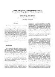
Witnesses. Using such transformations the processing of intersection points is deferred as
long as possible (lazy computation). The last possible point w(s,t) where an intersection
between two segments s and t has to be processed we call the witness of the intersection.
The witness w(s,t) is the lexicographically smallest segment endpoint that is located
within the closed wedge formed by the two intersecting segments s and t to the right
of the point of intersection (Figure 4.2). Note that each such wedge contains at least
two segment endpoints, namely the right endpoints of the two intersecting segments.
Therefore for any pair of intersecting segments its witness is well-defined.
s
t
Figure 4.2: The witness w(s,t) of an intersection s�t.
As a consequence, only the segment endpoints are EPs and the EPS can be determined
by lexicographic sorting during initialization. On the other hand, the SLS structure gets
more complicated because its order of segments does not necessarily reflect the order in
which the segments intersect the sweep line.
Invariants. The invariants of the algorithm have to take the relaxed notion of order into
account. Denote the sweep line by ℓ.
1. L is the sequence of segments from S intersecting ℓ; s appears before t in L =⇒ s
intersects ℓ above t or s intersects t and the witness of this intersection is to the
right of ℓ.
2. All intersections of segments from S whose witness is to the left of ℓ have been
reported.
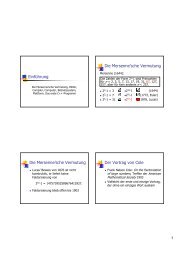
SLS Data Structure. The SLS structure consist of three levels. We use the fact that
segments of the same color do not interact, except by sharing endpoints possibly.
39
w

Chapter 4. Line Sweep CG 2012
1. Collect adjacent segments of the same color in bundles, stored as balanced search
trees. For each bundle store pointers to the topmost and bottommost segment.
(As the segments within one bundle are interior-disjoint, their order remains static
and thus correct under possible deformations due to lazy computation.)
2. All bundles are stored in a doubly linked list, sorted by y-coordinate.
3. All red bundles are stored in a balanced search tree (bundle tree).
Bundle
Tree
List
Figure 4.3: Graphical representation of the SLS data structure.
The search tree structure should support insert, delete, split and merge in (amortized)
logarithmic time each. For instance, splay trees [12] meet these requirements. (If you
have never heard about splay trees so far, you do not need to know for our purposes
here. Just treat them as a black box. However, you should take a note and read about
splay trees still. They are a fascinating data structure.)
EP handling. An EP p is processed as follows.
1. Localize p in bundle tree →�2 bundles containing p (all red bundles in between
must end at p). For the localization we use the pointers to the topmost and
bottommost segment within a bundle.
2. Localize p in�2red bundles found and split them at p. (If p is above the topmost
or below the bottommost segment of the bundle, there is no split.) All red bundles
are now either above, ending, or below with respect to p.
3. Localize p within the blue bundles by linear search.
4. Localize p in the�2blue bundles found and split them at p. (If p is above the
topmost or below the bottommost segment of the bundle, there is no split.) All
bundles are now either above, ending, or below with respect to p.
40

CG 2012 4.5. Red-Blue Intersections
5. Run through the list of bundles around p. More precisely, start from one of the
bundles containing p found in Step 1 and walk up in the doubly linked list of
bundles until two successive bundles (hence of opposite color) are both above p.
Similarly, walk down in the doubly linked list of bundles, until two successive
bundles are both below p. Handle all adjacent pairs of bundles (A,B) that are in
wrong order and report all pairs of segments as intersecting. (Exchange A and B
in the bundle list and merge them with their new neighbors.)
6. Report all pairs from begin(p)¢end(p) as intersecting.
7. Remove ending bundles and insert starting segments, sorted by slope and bundled
by color and possibly merge with the closest bundle above or below.
Remark: As both the red and the blue segments are interior-disjoint, at every EP there
can be at most one segment that passes through the EP. Should this happen, for the
purpose of EP processing split this segment into two, one ending and one starting at this
EP. But make sure to not report an intersection between the two parts!
Analysis. Sorting the EPS: O(n logn) time. Every EP generates a constant number of
tree searches and splits of O(logn) each. Every exchange in Step 5 generates at least
one intersection. New bundles are created only by inserting a new segment or by one
of the constant number of splits at an EP. Therefore O(n) bundles are created in total.
The total number of merge operations is O(n), as every merge kills one bundle and O(n)
bundles are created overall. The linear search in steps 3 and 5 can be charged either to
the ending bundle or—for continuing bundles—to the subsequent merge operation. In
summary, we have a runtime of O(n logn+k) and space usage is linear obviously.
Theorem 4.18 For two sets R and B, each consisting of interior-disjoint line segments
in R 2 , one can find all intersecting pairs of segments in O(n logn + k) time and
linear space, using predicates of maximum degree two. Here n = |R|+|B| and k is
the number of intersecting pairs.
Remarks. The first optimal algorithm for the red-blue intersection problem was published
in 1988 by Harry Mairson and Jorge Stolfi [7]. In 1994 Timothy Chan [3] described
a trapezoidal-sweep algorithm that uses predicates of degree three only. The approach
discussed above is due to Andrea Mantler and Jack Snoeyink [8] from 2000.
Exercise 4.19 Let S be a set of n segments each of which is either horizontal or
vertical. Describe an O(n logn) time and O(n) space algorithm that counts the
number of pairs in�S
2�that intersect.
41

Chapter 4. Line Sweep CG 2012
Questions
11. How can one test whether a polygon on n vertices is simple? Describe an
O(n logn) time algorithm.
12. How can one test whether two simple polygons on altogether n vertices intersect?
Describe an O(n logn) time algorithm.
13. How does the line sweep algorithm work that finds all k intersecting pairs
among n line segments in R 2 ? Describe the algorithm, using O((n + k) logn)
time and O(n) space. In particular, explain the data structures used, how event
points are handled, and how to cope with degeneracies.
14. Given two line segments s and t in R 2 whose endpoints have integer coordinates
in [0,2 b ); suppose s and t intersect in a single point q, what can you
say about the coordinates of q? Give a good (tight up to small additive number
of bits) upper bound on the size of these coordinates. (No need to prove tightness,
that is, give an example which achieves the bound.)
15. What is the degree of a predicate and why is it an important parameter? What
is the degree of the orientation test and the incircle test in R 2 ? Explain the
term and give two reasons for its relevance. Provide tight upper bounds for the
two predicates mentioned. (No need to prove tightness.)
16. What is the map overlay problem and how can it be solved optimally using
degree two predicates only? Give the problem definition and explain the term
“interior-disjoint”. Explain the bundle-sweep algorithm, in particular, the data
structures used, how an event point is processed, and the concept of witnesses.
References
[1] Ivan J. Balaban, An optimal algorithm for finding segment intersections. In
Proc. 11th Annu. ACM Sympos. Comput. Geom., pp. 211–219, 1995, URL
http://dx.doi.org/10.1145/220279.220302.
[2] Jon L. Bentley and Thomas A. Ottmann, Algorithms for reporting and counting
geometric intersections. IEEE Trans. Comput., C-28, 9, (1979), 643–647, URL
http://dx.doi.org/10.1109/TC.1979.1675432.
[3] Timothy M. Chan, A simple trapezoid sweep algorithm for reporting red/blue segment
intersections. In Proc. 6th Canad. Conf. Comput. Geom., pp. 263–268, 1994,
URL https://cs.uwaterloo.ca/~tmchan/red_blue.ps.gz.
[4] Bernard Chazelle, Triangulating a simple polygon in linear time. Discrete Comput.
Geom., 6, 5, (1991), 485–524, URL http://dx.doi.org/10.1007/BF02574703.
42

CG 2012 4.5. Red-Blue Intersections
[5] Bernard Chazelle and H. Edelsbrunner, An optimal algorithm for intersecting
line segments in the plane. J. ACM, 39, 1, (1992), 1–54, URL
http://dx.doi.org/10.1145/147508.147511.
[6] Kenneth L. Clarkson and Peter W. Shor, Applications of random sampling in
computational geometry, II. Discrete Comput. Geom., 4, (1989), 387–421, URL
http://dx.doi.org/10.1007/BF02187740.
[7] Harry G. Mairson and Jorge Stolfi, Reporting and counting intersections between
two sets of line segments. In R. A. Earnshaw, ed., Theoretical Foundations of
Computer Graphics and CAD, vol. 40 of NATO ASI Series F, pp. 307–325,
Springer-Verlag, Berlin, Germany, 1988.
[8] Andrea Mantler and Jack Snoeyink, Intersecting red and blue line segments
in optimal time and precision. In J. Akiyama, M. Kano, and
M. Urabe, eds., Proc. Japan Conf. Discrete Comput. Geom., vol. 2098
of Lecture Notes Comput. Sci., pp. 244–251, Springer Verlag, 2001, URL
http://dx.doi.org/10.1007/3-540-47738-1_23.
[9] Kurt Mehlhorn and Stefan Näher, Implementation of a sweep line algorithm for
the straight line segment intersection problem. Report MPI-I-94-160, Max-Planck-
Institut Inform., Saarbrücken, Germany, 1994.
[10] Ketan Mulmuley, A Fast Planar Partition Algorithm, I. J. Symbolic Comput., 10,
3-4, (1990), 253–280, URL http://dx.doi.org/10.1016/S0747-7171(08)80064-8.
[11] Ketan Mulmuley, A fast planar partition algorithm, II. J. ACM, 38, (1991), 74–103,
URL http://dx.doi.org/10.1145/102782.102785.
[12] Daniel D. Sleator and Robert E. Tarjan, Self-adjusting binary search trees. J. ACM,
32, 3, (1985), 652–686, URL http://dx.doi.org/10.1145/3828.3835.
43